Page Summary
-
Sparse tensor encoding enables automatic generation of sparse code from sparsity-agnostic representations, converting implicit sparsity to an explicit format.
-
It uses a map to define dimension and level specifications, including level-types (dense, compressed, loose_compressed, singleton, block2_4) and level-properties (nonunique, nonordered).
-
Level-expressions define an affine map between dimension and level coordinates, controlling how the sparse tensor is stored.
-
The encoding can optionally specify bitwidths for position and coordinate storage to optimize memory usage.
-
Examples of encodings include common formats like CSR, BSR, COO, and specialized formats like Nvidia's 2:4 structured sparsity and ELL.
Sparse tensor encoding is an attribute to encode information on sparsity properties of tensors, inspired by the TACO formalization of sparse tensors. This encoding is eventually used by a sparsifier pass to generate sparse code fully automatically from a sparsity-agnostic representation of the computation, i.e., an implicit sparse representation is converted to an explicit sparse representation where co-iterating loops operate on sparse storage formats rather than tensors with a sparsity encoding. Compiler passes that run before this sparsifier pass need to be aware of the semantics of tensor types with such a sparsity encoding.

In this encoding, we use dimension to refer to the axes of the semantic tensor, and level to refer to the axes of the actual storage format, i.e., the operational representation of the sparse tensor in memory. The number of dimensions is usually the same as the number of levels (such as CSR storage format). However, the encoding can also map dimensions to higher-order levels (for example, to encode a block-sparse BSR storage format) or to lower-order levels (for example, to linearize dimensions as a single level in the storage).
The encoding contains a map that provides the following:
- An ordered sequence of dimension specifications, each of which defines:
- the dimension-size (implicit from the tensor's dimension-shape)
- a dimension-expression
- An ordered sequence of level specifications, each of which includes a required
level-type, which defines how the level should be stored. Each level-type
consists of:
- a level-expression, which defines what is stored
- a level-format
- a collection of level-properties that apply to the level-format
Each level-expression is an affine expression over dimension-variables. Thus, the level-expressions collectively define an affine map from dimension-coordinates to level-coordinates. The dimension-expressions collectively define the inverse map, which only needs to be provided for elaborate cases where it cannot be inferred automatically.
Each dimension could also have an optional SparseTensorDimSliceAttr.
Within the sparse storage format, we refer to indices that are stored explicitly
as coordinates and offsets into the storage format as positions.
The supported level-formats are the following:
- dense : all entries along this level are stored
- compressed : only nonzeros along this level are stored
- loose_compressed : as compressed, but allows for free space between regions
- singleton : a variant of the compressed format, where coordinates have no siblings
- block2_4 : the compression uses a 2:4 encoding per 1x4 block
For a compressed level, each position interval is represented in a compact
way with a lowerbound pos(i) and an upperbound pos(i+1) - 1, which implies
that successive intervals must appear in order without any "holes" in between
them. The loose compressed format relaxes these constraints by representing each
position interval with a lowerbound lo(i) and an upperbound hi(i), which
allows intervals to appear in arbitrary order and with elbow room between them.
By default, each level-type has the property of being unique (no duplicate coordinates at that level) and ordered (coordinates appear sorted at that level). The following properties can be added to a level-format to change this default behavior:
- nonunique : duplicate coordinates may appear at the level
- nonordered : coordinates may appear in arbribratry order
In addition to the map, the following two fields are optional:
The required bitwidth for position storage (integral offsets into the sparse storage scheme). A narrow width reduces the memory footprint of overhead storage, as long as the width suffices to define the total required range (viz. the maximum number of stored entries over all indirection levels). The choices are
8,16,32,64, or, the default,0to indicate the native bitwidth.The required bitwidth for coordinate storage (the coordinates of stored entries). A narrow width reduces the memory footprint of overhead storage, as long as the width suffices to define the total required range (viz. the maximum value of each tensor coordinate over all levels). The choices are
8,16,32,64, or, the default,0to indicate a native bitwidth.
Examples
In the CSR(Compressed Sparse Row) format
shown below, the sparse tensor encoding
would be:
#CSR = #sparse_tensor.encoding<{
  map = (i, j) -> (i : dense, j : compressed)
}>
It indicates that the first dimension (row) maps to the first level,
which is a dense level, indicated by size 4. And the second dimension
(column) maps to the second level, indicated by positions array and
coordinates array. The value 3 ([1, 1] in the original matrix) is
represented by the offset from positions array (value 3's row number
is 1 in the original matrix as it's the second offset pair and its
column number resides in index [2 : 4) in the coordinates array). And in the
coordinates array, we can see that value 3's column number is 1 in the
original matrix.

For BSR(Block Sparse Row) format, the sparse tensor type is:
#BSR = #sparse_tensor.encoding<{
  map = (i, j) ->
    ( i floordiv 2 : dense
    , j floordiv 2 : compressed
    , i mod 2 : dense
    , j mod 2 : dense
    )
Consider the following sparse matrix, with 2x2 blocks:
Example 2x2 block storage:
 +-----+-----+-----+    +-----+-----+-----+
 | 1 2 | . . | 4 . |    | 1 2 |     | 4 0 |
 | . 3 | . . | . 5 |    | 0 3 |     | 0 5 |
 +-----+-----+-----+ => +-----+-----+-----+
 | . . | 6 7 | . . |    |     | 6 7 |     |
 | . . | 8 . | . . |    |     | 8 0 |     |
 +-----+-----+-----+    +-----+-----+-----+
which is ultimately stored in TACO-flavored format as
Stored as:
   positions[1]   : 0 2 3
   coordinates[1] : 0 2 1
   values         : 1.000000 2.000000 0.000000 3.000000
                    4.000000 0.000000 0.000000 5.000000
                    6.000000 7.000000 8.000000 0.000000
Which, incidentally, is literally the NVidia block format presented in the cuSparse documentation.
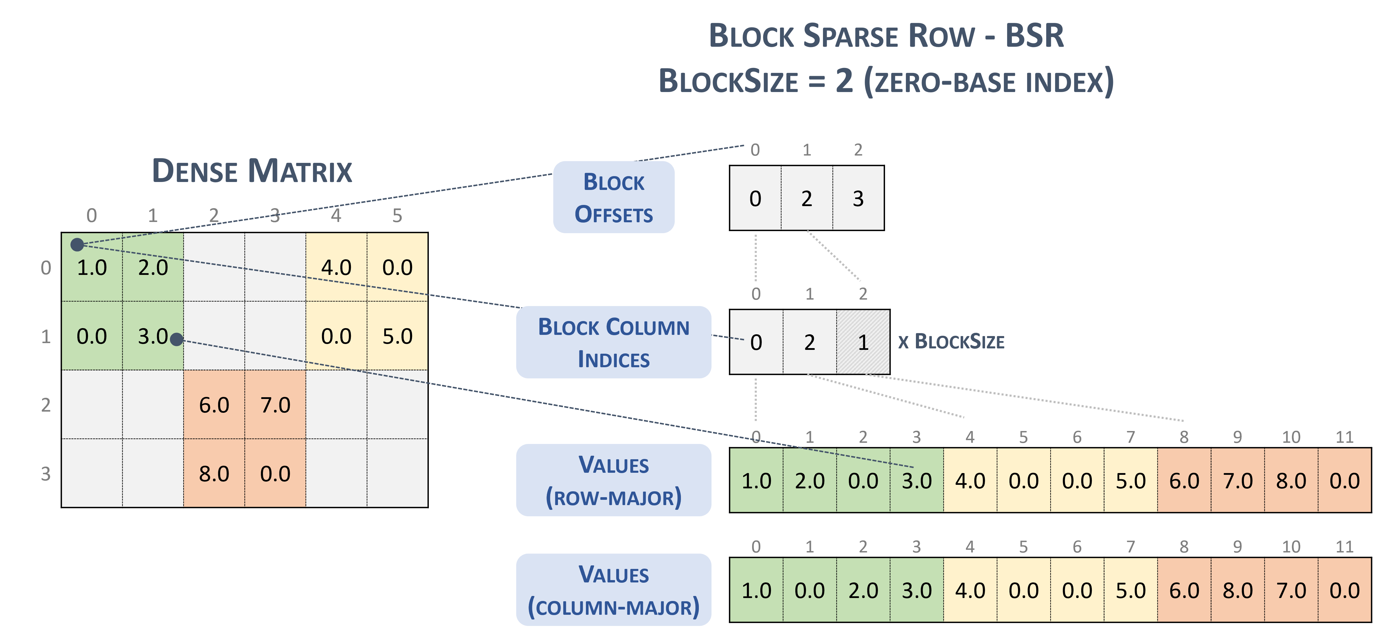
Block sparse row. (n.d.-b). Nvidia. https://docs.nvidia.com/cuda/cusparse/_images/bsr.png
We also support Nvidia's 2:4 structured sparsity.
The sparse tensor type for this is as follows:
#NV_24 = #sparse_tensor.encoding<{
  map = ( i, j ) -> ( i            : dense,
                      j floordiv 4 : dense,
                      j mod 4      : block2_4),
  crdWidth = 2  // 2-bits for each coordinate
}>
Given the sample matrix given in the NVidia documentation:
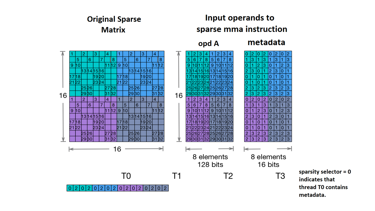
Sparse MMA storage example. (n.d.). Nvidia. https://docs.nvidia.com/cuda/parallel-thread-execution/index.html#warp-level-matrix-instructions-for-sparse-mma
MLIR now maps this matrix to an identical layout:
coordinates[2]  :
   0 2 0 2 0 2 0 2
   1 3 1 3 1 3 1 3
   0 1 2 3 0 1 2 3
   2 3 0 1 2 3 0 1
   0 1 0 1 0 1 0 1
   0 1 0 1 0 1 0 1
   2 3 2 3 2 3 2 3
   2 3 2 3 2 3 2 3
   0 2 0 2 0 2 0 2
   1 3 1 3 1 3 1 3
   0 1 2 3 0 1 2 3
   2 3 0 1 2 3 0 1
   0 1 0 1 0 1 0 1
   0 1 0 1 0 1 0 1
   2 3 2 3 2 3 2 3
   2 3 2 3 2 3 2 3
values :
  1.000000 2.000000 3.000000 4.000000 1.000000 2.000000 3.000000 4.000000
  5.000000 6.000000 7.000000 8.000000 5.000000 6.000000 7.000000 8.000000
  9.000000 10.000000 11.000000 12.000000 9.000000 10.000000 11.000000 12.000000
  13.000000 14.000000 15.000000 16.000000 13.000000 14.000000 15.000000 16.000000
  17.000000 18.000000 19.000000 20.000000 17.000000 18.000000 19.000000 20.000000
  21.000000 22.000000 23.000000 24.000000 21.000000 22.000000 23.000000 24.000000
  25.000000 26.000000 27.000000 28.000000 25.000000 26.000000 27.000000 28.000000
  29.000000 30.000000 31.000000 32.000000 29.000000 30.000000 31.000000 32.000000
More examples:
// Sparse vector.
#SparseVector = #sparse_tensor.encoding<{
  map = (i) -> (i : compressed)
}>
... tensor<?xf32, #SparseVector> ...

// Sorted coordinate scheme.
#SortedCOO = #sparse_tensor.encoding<{
  map = (i, j) -> (i : compressed(nonunique), j : singleton)
}>
... tensor<?x?xf64, #SortedCOO> ...

// Batched sorted coordinate scheme, with high encoding.
#BCOO = #sparse_tensor.encoding<{
  map = (i, j, k) -> (i : dense, j : compressed(nonunique, high), k : singleton)
}>
... tensor<10x10xf32, #BCOO> ...

// Compressed sparse row.
#CSR = #sparse_tensor.encoding<{
  map = (i, j) -> (i : dense, j : compressed)
}>
... tensor<100x100xbf16, #CSR> ...

// Doubly compressed sparse column storage with specific bitwidths.
#DCSC = #sparse_tensor.encoding<{
  map = (i, j) -> (j : compressed, i : compressed),
  posWidth = 32,
  crdWidth = 8
}>
... tensor<8x8xf64, #DCSC> ...

// Block sparse row storage (2x3 blocks).
#BSR = #sparse_tensor.encoding<{
  map = ( i, j ) ->
  ( i floordiv 2 : dense,
    j floordiv 3 : compressed,
    i mod 2      : dense,
    j mod 3      : dense
  )
}>
... tensor<20x30xf32, #BSR> ...

// Same block sparse row storage (2x3 blocks) but this time
// also with a redundant reverse mapping, which can be inferred.
#BSR_explicit = #sparse_tensor.encoding<{
  map = { ib, jb, ii, jj }
        ( i = ib * 2 + ii,
          j = jb * 3 + jj) ->
  ( ib = i floordiv 2 : dense,
    jb = j floordiv 3 : compressed,
    ii = i mod 2 : dense,
    jj = j mod 3 : dense)
}>
... tensor<20x30xf32, #BSR_explicit> ...

// ELL format.
// In the simple format for matrix, one array stores values and another
// array stores column indices. The arrays have the same number of rows
// as the original matrix, but only have as many columns as
// the maximum number of nonzeros on a row of the original matrix.
// There are many variants for ELL such as jagged diagonal scheme.
// To implement ELL, map provides a notion of "counting a
// dimension", where every stored element with the same coordinate
// is mapped to a new slice. For instance, ELL storage of a 2-d
// tensor can be defined with the mapping (i, j) -> (#i, i, j)
// using the notation of [Chou20]. Lacking the # symbol in MLIR's
// affine mapping, we use a free symbol c to define such counting,
// together with a constant that denotes the number of resulting
// slices. For example, the mapping [c](i, j) -> (c * 3 * i, i, j)
// with the level-types ["dense", "dense", "compressed"] denotes ELL
// storage with three jagged diagonals that count the dimension i.
#ELL = #sparse_tensor.encoding<{
  map = [c](i, j) -> (c * 3 * i : dense, i : dense, j : compressed)
}>
... tensor<?x?xf64, #ELL> ...

// CSR slice (offset = 0, size = 4, stride = 1 on the first dimension;
// offset = 0, size = 8, and a dynamic stride on the second dimension).
#CSR_SLICE = #sparse_tensor.encoding<{
  map = (i : #sparse_tensor<slice(0, 4, 1)>,
          j : #sparse_tensor<slice(0, 8, ?)>) ->
        (i : dense, j : compressed)
}>
... tensor<?x?xf64, #CSR_SLICE> ...