На этой странице представлены термины глоссария по основам машинного обучения. Чтобы просмотреть все термины глоссария, нажмите здесь .
А
точность
Количество правильных классификационных прогнозов, деленное на общее количество прогнозов. То есть:
Например, модель, сделавшая 40 правильных и 10 неправильных прогнозов, будет иметь точность:
Бинарная классификация предоставляет конкретные названия для различных категорий правильных и неправильных прогнозов . Таким образом, формула точности для бинарной классификации выглядит следующим образом:
где:
- TP — это количество истинно положительных результатов (правильных прогнозов).
- TN — это количество истинно отрицательных результатов (правильных предсказаний).
- FP — это количество ложноположительных результатов (неверных прогнозов).
- FN — это количество ложноотрицательных результатов (неверных прогнозов).
Сравните и сопоставьте точность с прецизией и полнотой .
Дополнительную информацию см. в разделе «Классификация: точность, полнота, прецизионность и связанные с ними показатели» в кратком курсе по машинному обучению.
функция активации
Функция, позволяющая нейронным сетям изучать нелинейные (сложные) взаимосвязи между признаками и меткой.
К популярным функциям активации относятся:
Графики функций активации никогда не представляют собой одну прямую линию. Например, график функции активации ReLU состоит из двух прямых линий:

График сигмоидной функции активации выглядит следующим образом:

Нажмите на значок, чтобы увидеть пример.
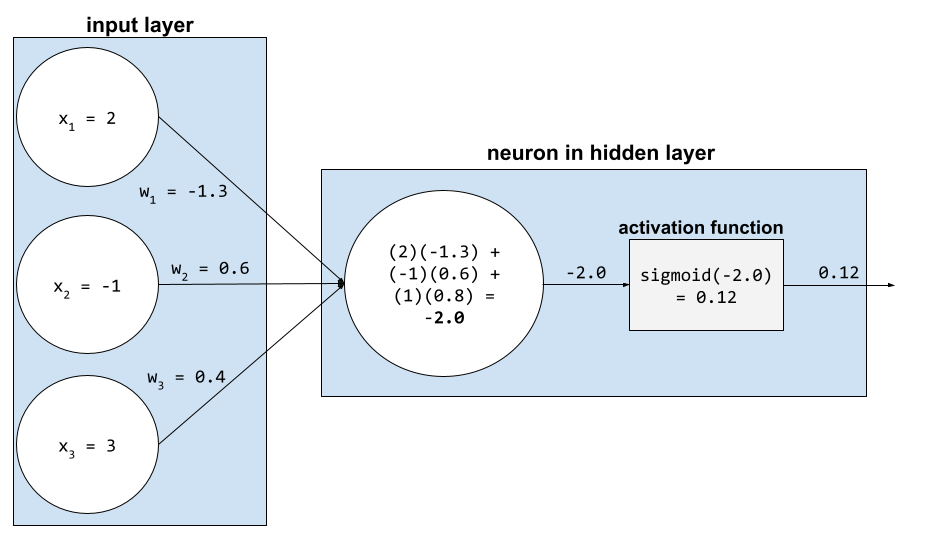
В нейронной сети функции активации обрабатывают взвешенную сумму всех входных сигналов нейрона . Для вычисления взвешенной суммы нейрон суммирует произведения соответствующих значений и весов. Например, предположим, что соответствующие входные сигналы для нейрона состоят из следующего:
| входное значение | входной вес |
| 2 | -1.3 |
| -1 | 0,6 |
| 3 | 0,4 |
weighted sum = (2)(-1.3) + (-1)(0.6) + (3)(0.4) = -2.0
Дополнительную информацию можно найти в разделе «Нейронные сети: функции активации» в кратком курсе по машинному обучению.
искусственный интеллект
Нечеловеческая программа или модель , способная решать сложные задачи. Например, программа или модель, переводящая текст, или программа или модель, определяющая заболевания по рентгеновским снимкам, — обе демонстрируют искусственный интеллект.
Формально машинное обучение является подразделом искусственного интеллекта. Однако в последние годы некоторые организации стали использовать термины «искусственный интеллект» и «машинное обучение» как взаимозаменяемые.
AUC (Площадь под ROC-кривой)
Число от 0,0 до 1,0, представляющее способность модели бинарной классификации разделять положительные и отрицательные классы . Чем ближе AUC к 1,0, тем лучше модель способна разделять классы.
Например, на следующем рисунке показана модель классификации , которая идеально разделяет положительные классы (зеленые овалы) от отрицательных классов (фиолетовые прямоугольники). Эта нереалистично идеальная модель имеет показатель AUC, равный 1,0:
Напротив, на следующем рисунке показаны результаты для модели классификации , которая генерировала случайные результаты. Для этой модели показатель AUC равен 0,5:
Да, у предыдущей модели показатель AUC равен 0,5, а не 0,0.
Большинство моделей находятся где-то между этими двумя крайностями. Например, следующая модель несколько разделяет положительные и отрицательные значения, и поэтому имеет AUC где-то между 0,5 и 1,0:
AUC игнорирует любые значения, которые вы задаете для порога классификации . Вместо этого AUC учитывает все возможные пороги классификации.
Нажмите на значок, чтобы узнать о взаимосвязи между AUC и ROC-кривыми.
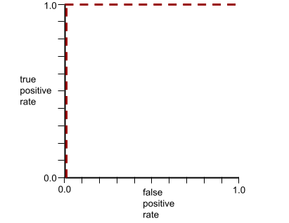
AUC представляет собой площадь под ROC-кривой . Например, ROC-кривая для модели, которая идеально разделяет положительные и отрицательные результаты, выглядит следующим образом:
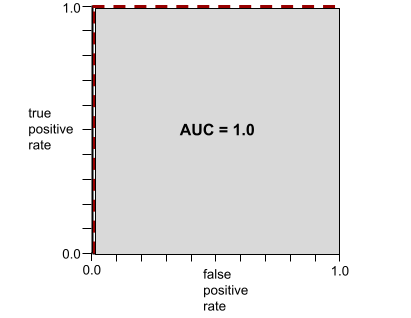
AUC — это площадь серой области на предыдущем рисунке. В этом необычном случае площадь — это просто длина серой области (1,0), умноженная на ширину серой области (1,0). Таким образом, произведение 1,0 и 1,0 дает AUC, равное ровно 1,0, что является максимально возможным значением AUC.
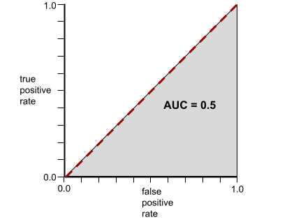
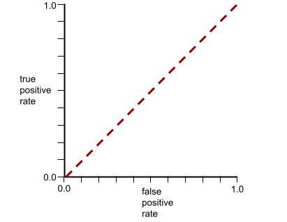
Напротив, ROC-кривая для модели классификации , которая вообще не может разделять классы, выглядит следующим образом. Площадь этой серой области составляет 0,5.
Типичная ROC-кривая выглядит примерно так:
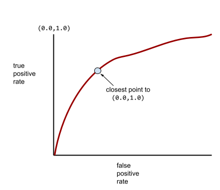
Вычисление площади под этой кривой вручную было бы трудоемким процессом, поэтому большинство значений AUC обычно рассчитываются программами.
Дополнительную информацию см. в разделе «Классификация: ROC и AUC в экспресс-курсе по машинному обучению».
Б
обратное распространение
Алгоритм, реализующий градиентный спуск в нейронных сетях .
Обучение нейронной сети включает в себя множество итераций следующего двухэтапного цикла:
- В процессе прямого прохода система обрабатывает пакет примеров для получения прогнозов. Система сравнивает каждый прогноз с каждым значением метки . Разница между прогнозом и значением метки представляет собой ошибку для данного примера. Система суммирует ошибки для всех примеров, чтобы вычислить общую ошибку для текущего пакета.
- В процессе обратного распространения ошибки система уменьшает потери, корректируя веса всех нейронов во всех скрытых слоях .
Нейронные сети часто содержат множество нейронов в различных скрытых слоях. Каждый из этих нейронов вносит свой вклад в общую функцию потерь. Обратное распространение ошибки определяет, следует ли увеличивать или уменьшать веса, применяемые к конкретным нейронам.
Скорость обучения — это множитель, который регулирует степень увеличения или уменьшения каждого веса при каждом обратном проходе. Высокая скорость обучения будет увеличивать или уменьшать каждый вес сильнее, чем низкая скорость обучения.
В терминах математического анализа, обратное распространение ошибки реализует правило цепочки из математического анализа. То есть, обратное распространение ошибки вычисляет частную производную ошибки по каждому параметру.
Несколько лет назад специалистам по машинному обучению приходилось писать код для реализации обратного распространения ошибки. Современные API для машинного обучения, такие как Keras, теперь реализуют обратное распространение ошибки автоматически. Уф!
Для получения более подробной информации см. раздел «Нейронные сети в кратком курсе по машинному обучению».
партия
Набор примеров, используемых в одной итерации обучения. Размер пакета определяет количество примеров в пакете.
См. раздел «Эпоха» для объяснения того, как пакет данных соотносится с эпохой.
Для получения более подробной информации см. статью «Линейная регрессия: гиперпараметры в машинном обучении».
размер партии
Количество примеров в пакете . Например, если размер пакета равен 100, то модель обрабатывает 100 примеров за итерацию .
Ниже представлены популярные стратегии определения размера партии:
- Стохастический градиентный спуск (SGD) , в котором размер пакета равен 1.
- Полный пакет (Full batch) — это стратегия, в которой размер пакета равен количеству примеров во всем обучающем наборе данных . Например, если обучающий набор содержит миллион примеров, то размер пакета будет равен миллиону примеров. Стратегия полного пакета обычно неэффективна.
- Мини-партии, размер партии которых обычно составляет от 10 до 1000 единиц. Мини-партии, как правило, являются наиболее эффективной стратегией.
Дополнительную информацию см. ниже:
- Системы машинного обучения для производственных целей: статический и динамический вывод в кратком курсе по машинному обучению.
- Руководство по настройке глубокого обучения .
предвзятость (этика/справедливость)
1. Стереотипизация, предвзятость или фаворитизм по отношению к одним вещам, людям или группам по сравнению с другими. Эти предубеждения могут влиять на сбор и интерпретацию данных, проектирование системы и взаимодействие пользователей с ней. К таким формам предвзятости относятся:
- предвзятость автоматизации
- предвзятость подтверждения
- Предвзятость экспериментатора
- предвзятость групповой атрибуции
- неявная предвзятость
- предвзятость внутри группы
- смещение однородности внешней группы
2. Систематическая ошибка, возникающая в результате процедуры выборки или составления отчета. К таким формам смещения относятся:
- смещение охвата
- смещение, вызванное отсутствием ответа
- предвзятость участия
- предвзятость в репортажах
- смещение выборки
- предвзятость отбора
Не следует путать с термином «смещение» в моделях машинного обучения или смещением прогнозирования .
Дополнительную информацию см. в разделе «Справедливость: виды предвзятости в экспресс-курсе по машинному обучению».
смещение (математика) или термин, обозначающий смещение
Пересечение или смещение относительно начала координат. Смещение — это параметр в моделях машинного обучения, который обозначается одним из следующих символов:
- б
- w 0
Например, смещение обозначается буквой b в следующей формуле:
В простой двумерной прямой смещение просто означает «пересечение с осью Y». Например, смещение прямой на следующем рисунке равно 2.
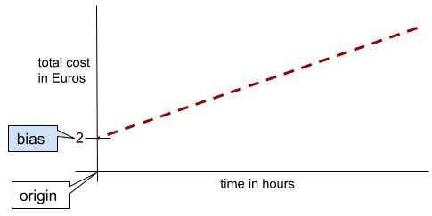
Смещение существует потому, что не все модели начинаются с начала координат (0,0). Например, предположим, что вход в парк развлечений стоит 2 евро, и дополнительно 0,5 евро за каждый час пребывания посетителя. Следовательно, модель, отображающая общую стоимость, имеет смещение, равное 2, поскольку минимальная стоимость составляет 2 евро.
Предвзятость не следует путать с предвзятостью в этике и справедливости или с предвзятостью прогнозирования .
Для получения более подробной информации см. «Линейная регрессия в машинном обучении: краткий курс».
бинарная классификация
Тип задачи классификации , в которой предсказывается один из двух взаимоисключающих классов:
Например, следующие две модели машинного обучения выполняют бинарную классификацию:
- Модель, определяющая, являются ли электронные письма спамом (положительный класс) или не спамом (отрицательный класс).
- Модель, которая оценивает медицинские симптомы, чтобы определить, есть ли у человека определенное заболевание (положительный класс) или нет (отрицательный класс).
В отличие от многоклассовой классификации .
См. также логистическую регрессию и порог классификации .
Дополнительную информацию см. в разделе «Краткий курс по классификации в машинном обучении».
ведро
Преобразование одного признака в несколько бинарных признаков, называемых интервалами или ячейками , обычно на основе диапазона значений. Обрезанный признак, как правило, является непрерывным признаком .
Например, вместо представления температуры в виде единого непрерывного значения с плавающей запятой, можно разделить диапазоны температур на дискретные интервалы, такие как:
- Температура <= 10 градусов Цельсия будет считаться "холодной".
- Температура от 11 до 24 градусов Цельсия соответствует "умеренному" климату.
- Температура выше или равная 25 градусам Цельсия будет считаться "теплой" температурой.
Модель будет обрабатывать каждое значение в одной и той же категории одинаково. Например, значения 13 и 22 находятся в категории умеренного климата, поэтому модель обрабатывает эти два значения одинаково.
Дополнительную информацию см. в разделе «Числовые данные: биннинг в машинном обучении» (краткий курс).
С
категориальные данные
Признаки, имеющие определенный набор возможных значений. Например, рассмотрим категориальный признак с именем traffic-light-state , который может принимать только одно из следующих трех возможных значений:
-
red -
yellow -
green
Представляя traffic-light-state как категориальный признак, модель может изучить различное влияние red , green и yellow на поведение водителя.
Категориальные признаки иногда называют дискретными признаками .
Сравните с числовыми данными .
Дополнительную информацию см. в разделе «Работа с категориальными данными» в кратком курсе по машинному обучению.
сорт
Категория, к которой может относиться метка . Например:
- В модели бинарной классификации , предназначенной для обнаружения спама, два класса могут быть спамом , а два — не спамом .
- В многоклассовой модели классификации , определяющей породы собак, классами могут быть пудель , бигль , мопс и так далее.
Классификационная модель предсказывает класс. В отличие от неё, регрессионная модель предсказывает число, а не класс.
Дополнительную информацию см. в разделе «Краткий курс по классификации в машинном обучении».
модель классификации
Модель , предсказание которой представляет собой класс . Например, все следующие модели являются моделями классификации:
- Модель, которая предсказывает язык входного предложения (французский? испанский? итальянский?).
- Модель, которая предсказывает виды деревьев (клен? дуб? баобаб?).
- Модель, которая предсказывает положительный или отрицательный класс для конкретного медицинского состояния.
В отличие от этого, регрессионные модели прогнозируют числа, а не классы.
К распространенным типам моделей классификации относятся:
порог классификации
В бинарной классификации пороговое значение — это число от 0 до 1, которое преобразует исходные данные модели логистической регрессии в предсказание либо положительного , либо отрицательного класса . Следует отметить, что пороговое значение классификации выбирается человеком, а не обучающей моделью.
Модель логистической регрессии выдает исходное значение от 0 до 1. Затем:
- Если это исходное значение превышает пороговое значение классификации, то прогнозируется положительная принадлежность к классу.
- Если это исходное значение меньше порогового значения классификации, то прогнозируется отрицательный класс.
Например, предположим, что пороговое значение классификации равно 0,8. Если исходное значение равно 0,9, то модель предсказывает положительный класс. Если исходное значение равно 0,7, то модель предсказывает отрицательный класс.
Выбор порогового значения классификации оказывает существенное влияние на количество ложноположительных и ложноотрицательных результатов .
Более подробную информацию см. в разделе «Пороги и матрица ошибок» в кратком курсе по машинному обучению.
классификатор
Неформальное название модели классификации .
несбалансированный по классам набор данных
Набор данных для классификации , в котором общее количество меток каждого класса значительно различается. Например, рассмотрим набор данных для бинарной классификации , в котором две метки разделены следующим образом:
- 1 000 000 негативных этикеток
- 10 положительных отзывов
Соотношение отрицательных и положительных меток составляет 100 000 к 1, поэтому это набор данных с несбалансированным распределением классов.
Напротив, следующий набор данных является сбалансированным по классам, поскольку отношение отрицательных меток к положительным относительно близко к 1:
- 517 негативных меток
- 483 положительных отзыва
Многоклассовые наборы данных также могут быть несбалансированными по классам. Например, следующий набор данных для многоклассовой классификации также является несбалансированным по классам, поскольку одна метка содержит гораздо больше примеров, чем две другие:
- 1 000 000 этикеток с классом «зеленый»
- 200 этикеток с классом «фиолетовый»
- 350 этикеток с классом "оранжевый"
Обучение на несбалансированных по классам наборах данных может представлять особые трудности. Подробнее см. раздел «Несбалансированные наборы данных» в кратком курсе по машинному обучению.
См. также энтропию , мажоритарный класс и миноритарный класс .
обрезка
Метод обработки выбросов, включающий один или оба из следующих действий:
- Снижение значений признаков , превышающих максимальный пороговый уровень, до этого максимального порогового значения.
- Увеличение значений характеристик, которые ниже минимального порогового значения, до этого минимального порогового значения.
Например, предположим, что менее 0,5% значений для определенного параметра выходят за пределы диапазона 40–60. В этом случае можно сделать следующее:
- Обрежьте все значения, превышающие 60 (максимальный порог), до значения ровно 60.
- Обрежьте все значения ниже 40 (минимальный порог) до значения ровно 40.
Выбросы могут навредить моделям, иногда вызывая переполнение весов во время обучения. Некоторые выбросы также могут значительно ухудшить такие показатели, как точность . Ограничение — распространенный метод для минимизации ущерба.
Ограничение градиента заставляет значения градиента находиться в заданном диапазоне во время обучения.
Дополнительную информацию см. в разделе «Числовые данные: нормализация в машинном обучении» (краткий курс).
матрица ошибок
Таблица размером NxN, в которой суммируется количество правильных и неправильных предсказаний, сделанных моделью классификации . Например, рассмотрим следующую матрицу ошибок для модели бинарной классификации :
| Опухоль (прогнозируемая) | Неопухолевый (прогнозируемый) | |
|---|---|---|
| Опухоль (эталонные данные) | 18 (ТП) | 1 (FN) |
| Нетуморальный (эталонный) | 6 (FP) | 452 (ТН) |
Представленная выше матрица ошибок показывает следующее:
- Из 19 прогнозов, в которых в качестве истинного диагноза была указана опухоль, модель правильно классифицировала 18 и неправильно классифицировала 1.
- Из 458 прогнозов, в которых истинное значение указывало на отсутствие опухоли, модель правильно классифицировала 452 случая и неправильно — 6.
Матрица ошибок для задачи многоклассовой классификации может помочь выявить закономерности ошибок. Например, рассмотрим следующую матрицу ошибок для модели многоклассовой классификации с тремя классами, которая классифицирует три разных типа ирисов (Virginica, Versicolor и Setosa). Когда истинным значением был Virginica, матрица ошибок показывает, что модель гораздо чаще ошибочно предсказывала Versicolor, чем Setosa:
| Сетоса (прогнозируемая) | Разноцветный (прогнозируемый) | Вирджиния (прогнозируется) | |
|---|---|---|---|
| Сетоса (эталонные данные) | 88 | 12 | 0 |
| Versicolor (эталонные данные) | 6 | 141 | 7 |
| Вирджиния (на основе реальных данных) | 2 | 27 | 109 |
В качестве еще одного примера, матрица ошибок может показать, что модель, обученная распознавать рукописные цифры, склонна ошибочно предсказывать 9 вместо 4 или ошибочно предсказывать 1 вместо 7.
Матрица ошибок содержит достаточно информации для расчета различных показателей эффективности, включая точность и полноту .
непрерывная функция
Параметр типа "число с плавающей запятой" с бесконечным диапазоном возможных значений, например, температура или вес.
В отличие от дискретных признаков .
конвергенция
Состояние, при котором значения функции потерь изменяются очень незначительно или не изменяются вовсе с каждой итерацией . Например, следующая кривая потерь указывает на сходимость примерно на 700 итерациях:
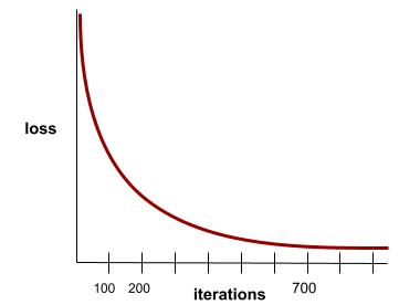
Модель сходится , когда дополнительное обучение не улучшает её.
В глубоком обучении значения функции потерь иногда остаются постоянными или почти постоянными на протяжении многих итераций, прежде чем, наконец, начать снижаться. В течение длительного периода постоянных значений функции потерь может возникнуть ложное ощущение сходимости.
См. также раннюю остановку .
Дополнительную информацию см. в разделе «Сходимость модели и кривые потерь» в «Кратком курсе по машинному обучению».
Д
DataFrame
Популярный тип данных в pandas для представления наборов данных в памяти.
DataFrame аналогичен таблице или электронной таблице. Каждый столбец DataFrame имеет имя (заголовок), а каждая строка идентифицируется уникальным номером.
Каждый столбец в DataFrame имеет структуру двумерного массива, за исключением того, что каждому столбцу может быть присвоен свой собственный тип данных.
См. также официальную справочную страницу pandas.DataFrame .
набор данных или набор данных
Набор необработанных данных, обычно (но не исключительно) организованных в одном из следующих форматов:
- электронная таблица
- файл в формате CSV (значения, разделенные запятыми)
глубокая модель
Нейронная сеть, содержащая более одного скрытого слоя .
Глубокая модель также называется глубокой нейронной сетью .
Сравните с широкой моделью .
плотный элемент
Характеристика , при которой большинство или все значения ненулевые, обычно это тензор с плавающей запятой. Например, следующий тензор из 10 элементов является плотным, поскольку 9 его значений ненулевые:
| 8 | 3 | 7 | 5 | 2 | 4 | 0 | 4 | 9 | 6 |
В отличие от скудных характеристик .
глубина
Сумма следующих величин в нейронной сети :
- количество скрытых слоев
- количество выходных слоев , которое обычно равно 1.
- количество любых слоев встраивания
Например, нейронная сеть с пятью скрытыми слоями и одним выходным слоем имеет глубину 6.
Обратите внимание, что входной слой не влияет на глубину.
дискретная функция
Признак с конечным множеством возможных значений. Например, признак, значения которого могут быть только «животное» , «растение» или «минерал» , является дискретным (или категориальным) признаком.
В отличие от непрерывной характеристики .
динамический
Что-либо, выполняемое часто или непрерывно. Термины «динамичный» и «онлайн» являются синонимами в машинном обучении. Ниже приведены распространенные примеры использования терминов «динамичный» и «онлайн» в машинном обучении:
- Динамическая модель (или онлайн-модель ) — это модель, которая часто или непрерывно переобучается.
- Динамическое обучение (или онлайн-обучение ) — это процесс обучения, проводимый часто или непрерывно.
- Динамический вывод (или онлайн-вывод ) — это процесс генерации прогнозов по запросу.
динамическая модель
Динамическая модель — это модель , которая часто (возможно, даже непрерывно) переобучается. Это «модель, обучающаяся на протяжении всей жизни», которая постоянно адаптируется к изменяющимся данным. Динамическую модель также называют онлайн-моделью .
Сравните со статической моделью .
Е
ранняя остановка
Метод регуляризации , предполагающий завершение обучения до того, как функция потерь на обучающем наборе данных перестанет уменьшаться. При ранней остановке обучение модели намеренно прекращается, когда функция потерь на проверочном наборе данных начинает увеличиваться, то есть когда производительность обобщения ухудшается.
Сравните с ранним выходом .
встраиваемый слой
Специальный скрытый слой , который обучается на многомерном категориальном признаке, постепенно изучая вектор встраивания меньшей размерности. Слой встраивания позволяет нейронной сети обучаться гораздо эффективнее, чем при обучении только на многомерном категориальном признаке.
Например, на Земле в настоящее время произрастает около 73 000 видов деревьев. Предположим, что вид дерева является характеристикой вашей модели, поэтому входной слой вашей модели включает в себя вектор one-hot длиной 73 000 элементов. Например, baobab может быть представлен примерно так:
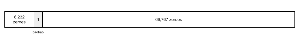
Массив из 73 000 элементов очень длинный. Если не добавить слой встраивания к модели, обучение будет очень трудоемким из-за необходимости умножения на 72 999 нулей. Возможно, вы выберете слой встраивания, состоящий из 12 измерений. В результате слой встраивания будет постепенно обучаться новому вектору встраивания для каждого вида деревьев.
В некоторых ситуациях хеширование является разумной альтернативой слою встраивания.
Для получения более подробной информации см. краткий курс по встраиванию данных в машинное обучение.
эпоха
Полный цикл обучения по всему обучающему набору данных , при котором каждый пример обрабатывается один раз.
Одна эпоха соответствует N / размеру пакета итераций обучения, где N — общее количество примеров.
Например, предположим следующее:
- Набор данных состоит из 1000 примеров.
- Размер партии составляет 50 экземпляров.
Таким образом, для одной эпохи требуется 20 итераций:
1 epoch = (N/batch size) = (1,000 / 50) = 20 iterations
Для получения более подробной информации см. статью «Линейная регрессия: гиперпараметры в машинном обучении».
пример
Значения одной строки признаков и, возможно, метка . Примеры в контролируемом обучении делятся на две общие категории:
- Размеченный пример состоит из одного или нескольких признаков и метки. Размеченные примеры используются во время обучения.
- Пример без меток состоит из одного или нескольких признаков, но не имеет метки. Примеры без меток используются при выводе результатов.
Например, предположим, вы обучаете модель для определения влияния погодных условий на результаты тестов учащихся. Вот три примера с обозначениями:
| Функции | Этикетка | ||
|---|---|---|---|
| Температура | Влажность | Давление | Результат теста |
| 15 | 47 | 998 | Хороший |
| 19 | 34 | 1020 | Отличный |
| 18 | 92 | 1012 | Бедный |
Вот три примера без подписей:
| Температура | Влажность | Давление | |
|---|---|---|---|
| 12 | 62 | 1014 | |
| 21 | 47 | 1017 | |
| 19 | 41 | 1021 |
Строка набора данных обычно является исходным материалом для примера. То есть пример, как правило, представляет собой подмножество столбцов набора данных. Кроме того, признаки в примере могут также включать синтетические признаки , такие как перекрестные признаки .
Более подробную информацию см. в разделе «Обучение с учителем» курса «Введение в машинное обучение».
Ф
ложноотрицательный результат (FN)
Пример, в котором модель ошибочно предсказывает отрицательный класс . Например, модель предсказывает, что конкретное электронное письмо не является спамом (отрицательный класс), но на самом деле это письмо является спамом .
ложноположительный результат (FP)
Пример, в котором модель ошибочно предсказывает положительный класс . Например, модель предсказывает, что конкретное электронное письмо является спамом (положительный класс), но на самом деле это электронное письмо не является спамом .
Более подробную информацию см. в разделе «Пороги и матрица ошибок» в кратком курсе по машинному обучению.
Частота ложноположительных результатов (FPR)
Доля фактически отрицательных примеров, для которых модель ошибочно предсказала положительный класс. Следующая формула вычисляет частоту ложноположительных результатов:
Показатель ложноположительных результатов отображается по оси X на ROC-кривой .
Дополнительную информацию см. в разделе «Классификация: ROC и AUC в экспресс-курсе по машинному обучению».
особенность
Входная переменная для модели машинного обучения. Пример состоит из одного или нескольких признаков. Например, предположим, вы обучаете модель для определения влияния погодных условий на результаты тестов учащихся. В следующей таблице показаны три примера, каждый из которых содержит три признака и одну метку:
| Функции | Этикетка | ||
|---|---|---|---|
| Температура | Влажность | Давление | Результат теста |
| 15 | 47 | 998 | 92 |
| 19 | 34 | 1020 | 84 |
| 18 | 92 | 1012 | 87 |
Сравните с этикеткой .
Более подробную информацию см. в разделе «Обучение с учителем» курса «Введение в машинное обучение».
кросс функций
Синтетический признак , сформированный путем "пересечения" категориальных или сгруппированных признаков.
Например, рассмотрим модель «прогнозирования настроения», которая представляет температуру в одном из следующих четырех диапазонов:
-
freezing -
chilly -
temperate -
warm
И представляет собой скорость ветра в одной из следующих трех категорий:
-
still -
light -
windy
Без перекрестного сопоставления признаков линейная модель обучается независимо на каждом из семи предыдущих различных сегментов. Таким образом, модель обучается, например, freezing независимо от обучения, например, windy .
В качестве альтернативы можно создать комбинацию параметров температуры и скорости ветра. Эта синтетическая характеристика будет иметь следующие 12 возможных значений:
-
freezing-still -
freezing-light -
freezing-windy -
chilly-still -
chilly-light -
chilly-windy -
temperate-still -
temperate-light -
temperate-windy -
warm-still -
warm-light -
warm-windy
Благодаря сопоставлению признаков модель может изучать различия в настроении в freezing-windy день и в freezing-still день.
Если создать синтетический признак из двух признаков, каждый из которых имеет множество различных категорий, то результирующее скрещивание признаков будет иметь огромное количество возможных комбинаций. Например, если один признак имеет 1000 категорий, а другой — 2000, то результирующее скрещивание признаков будет иметь 2 000 000 категорий.
Формально, крест — это декартово произведение .
Метод перекрестных проверок признаков в основном используется в линейных моделях и редко применяется в нейронных сетях.
Дополнительную информацию см. в разделе «Категориальные данные: Пересечение признаков» в кратком курсе по машинному обучению.
разработка функций
Процесс, включающий следующие этапы:
- Определение того, какие признаки могут быть полезны при обучении модели.
- Преобразование исходных данных из набора данных в эффективные версии этих признаков.
For example, you might determine that temperature might be a useful feature. Then, you might experiment with bucketing to optimize what the model can learn from different temperature ranges.
Feature engineering is sometimes called feature extraction or featurization .
See Numerical data: How a model ingests data using feature vectors in Machine Learning Crash Course for more information.
набор функций
The group of features your machine learning model trains on. For example, a simple feature set for a model that predicts housing prices might consist of postal code, property size, and property condition.
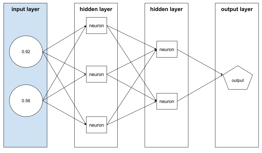
feature vector
The array of feature values comprising an example . The feature vector is input during training and during inference . For example, the feature vector for a model with two discrete features might be:
[0.92, 0.56]
Each example supplies different values for the feature vector, so the feature vector for the next example could be something like:
[0.73, 0.49]
Feature engineering determines how to represent features in the feature vector. For example, a binary categorical feature with five possible values might be represented with one-hot encoding . In this case, the portion of the feature vector for a particular example would consist of four zeroes and a single 1.0 in the third position, as follows:
[0.0, 0.0, 1.0, 0.0, 0.0]
As another example, suppose your model consists of three features:
- a binary categorical feature with five possible values represented with one-hot encoding; for example:
[0.0, 1.0, 0.0, 0.0, 0.0] - another binary categorical feature with three possible values represented with one-hot encoding; for example:
[0.0, 0.0, 1.0] - a floating-point feature; for example:
8.3.
In this case, the feature vector for each example would be represented by nine values. Given the example values in the preceding list, the feature vector would be:
0.0
1.0
0.0
0.0
0.0
0.0
0.0
1.0
8.3
See Numerical data: How a model ingests data using feature vectors in Machine Learning Crash Course for more information.
петля обратной связи
In machine learning, a situation in which a model's predictions influence the training data for the same model or another model. For example, a model that recommends movies will influence the movies that people see, which will then influence subsequent movie recommendation models.
See Production ML systems: Questions to ask in Machine Learning Crash Course for more information.
Г
обобщение
A model's ability to make correct predictions on new, previously unseen data. A model that can generalize is the opposite of a model that is overfitting .
See Generalization in Machine Learning Crash Course for more information.
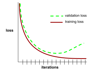
generalization curve
A plot of both training loss and validation loss as a function of the number of iterations .
A generalization curve can help you detect possible overfitting . For example, the following generalization curve suggests overfitting because validation loss ultimately becomes significantly higher than training loss.
See Generalization in Machine Learning Crash Course for more information.
градиентный спуск
A mathematical technique to minimize loss . Gradient descent iteratively adjusts weights and biases , gradually finding the best combination to minimize loss.
Gradient descent is older—much, much older—than machine learning.
See the Linear regression: Gradient descent in Machine Learning Crash Course for more information.
эталонные данные
Реальность.
The thing that actually happened.
For example, consider a binary classification model that predicts whether a student in their first year of university will graduate within six years. Ground truth for this model is whether or not that student actually graduated within six years.
ЧАС
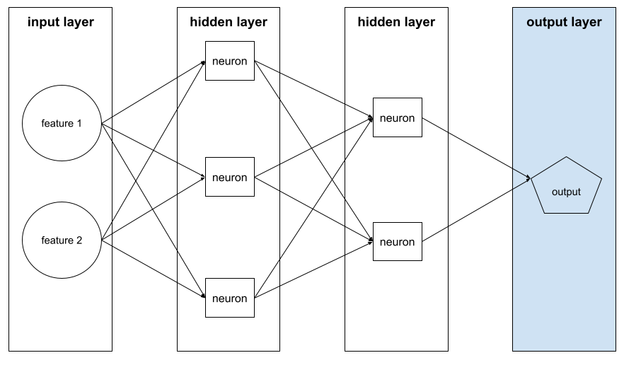
скрытый слой
A layer in a neural network between the input layer (the features) and the output layer (the prediction). Each hidden layer consists of one or more neurons . For example, the following neural network contains two hidden layers, the first with three neurons and the second with two neurons:
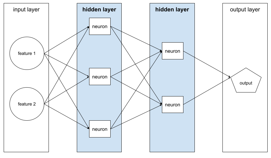
A deep neural network contains more than one hidden layer. For example, the preceding illustration is a deep neural network because the model contains two hidden layers.
See Neural networks: Nodes and hidden layers in Machine Learning Crash Course for more information.
гиперпараметр
The variables that you or a hyperparameter tuning serviceadjust during successive runs of training a model. For example, learning rate is a hyperparameter. You could set the learning rate to 0.01 before one training session. If you determine that 0.01 is too high, you could perhaps set the learning rate to 0.003 for the next training session.
In contrast, parameters are the various weights and bias that the model learns during training.
See Linear regression: Hyperparameters in Machine Learning Crash Course for more information.
я
independently and identically distributed (iid)
Data drawn from a distribution that doesn't change, and where each value drawn doesn't depend on values that have been drawn previously. An iid is the ideal gas of machine learning—a useful mathematical construct but almost never exactly found in the real world. For example, the distribution of visitors to a web page may be iid over a brief window of time; that is, the distribution doesn't change during that brief window and one person's visit is generally independent of another's visit. However, if you expand that window of time, seasonal differences in the web page's visitors may appear.
See also nonstationarity .
вывод
In traditional machine learning, the process of making predictions by applying a trained model to unlabeled examples . See Supervised Learning in the Intro to ML course to learn more.
In large language models , inference is the process of using a trained model to generate a response to an input prompt .
Inference has a somewhat different meaning in statistics. See the Wikipedia article on statistical inference for details.
input layer
The layer of a neural network that holds the feature vector . That is, the input layer provides examples for training or inference . For example, the input layer in the following neural network consists of two features:

интерпретируемость
The ability to explain or to present an ML model's reasoning in understandable terms to a human.
Most linear regression models, for example, are highly interpretable. (You merely need to look at the trained weights for each feature.) Decision forests are also highly interpretable. Some models, however, require sophisticated visualization to become interpretable.
You can use the Learning Interpretability Tool (LIT) to interpret ML models.
итерация
A single update of a model's parameters—the model's weights and biases —during training . The batch size determines how many examples the model processes in a single iteration. For instance, if the batch size is 20, then the model processes 20 examples before adjusting the parameters.
When training a neural network , a single iteration involves the following two passes:
- A forward pass to evaluate loss on a single batch.
- A backward pass ( backpropagation ) to adjust the model's parameters based on the loss and the learning rate.
See Gradient descent in Machine Learning Crash Course for more information.
Л
L 0 regularization
A type of regularization that penalizes the total number of nonzero weights in a model. For example, a model having 11 nonzero weights would be penalized more than a similar model having 10 nonzero weights.
L 0 regularization is sometimes called L0-norm regularization .
L 1 loss
A loss function that calculates the absolute value of the difference between actual label values and the values that a model predicts. For example, here's the calculation of L 1 loss for a batch of five examples :
| Actual value of example | Model's predicted value | Absolute value of delta |
|---|---|---|
| 7 | 6 | 1 |
| 5 | 4 | 1 |
| 8 | 11 | 3 |
| 4 | 6 | 2 |
| 9 | 8 | 1 |
| 8 = L 1 loss | ||
L 1 loss is less sensitive to outliers than L 2 loss .
The Mean Absolute Error is the average L 1 loss per example.
See Linear regression: Loss in Machine Learning Crash Course for more information.
L 1 regularization
A type of regularization that penalizes weights in proportion to the sum of the absolute value of the weights. L 1 regularization helps drive the weights of irrelevant or barely relevant features to exactly 0 . A feature with a weight of 0 is effectively removed from the model.
Contrast with L 2 regularization .
Потеря L 2
A loss function that calculates the square of the difference between actual label values and the values that a model predicts. For example, here's the calculation of L 2 loss for a batch of five examples :
| Actual value of example | Model's predicted value | Square of delta |
|---|---|---|
| 7 | 6 | 1 |
| 5 | 4 | 1 |
| 8 | 11 | 9 |
| 4 | 6 | 4 |
| 9 | 8 | 1 |
| 16 = L 2 loss | ||
Due to squaring, L 2 loss amplifies the influence of outliers . That is, L 2 loss reacts more strongly to bad predictions than L 1 loss . For example, the L 1 loss for the preceding batch would be 8 rather than 16. Notice that a single outlier accounts for 9 of the 16.
Regression models typically use L 2 loss as the loss function.
The Mean Squared Error is the average L 2 loss per example. Squared loss is another name for L 2 loss.
See Logistic regression: Loss and regularization in Machine Learning Crash Course for more information.
L 2 regularization
A type of regularization that penalizes weights in proportion to the sum of the squares of the weights. L 2 regularization helps drive outlier weights (those with high positive or low negative values) closer to 0 but not quite to 0 . Features with values very close to 0 remain in the model but don't influence the model's prediction very much.
L 2 regularization always improves generalization in linear models .
Contrast with L 1 regularization .
See Overfitting: L2 regularization in Machine Learning Crash Course for more information.
этикетка
In supervised machine learning , the "answer" or "result" portion of an example .
Each labeled example consists of one or more features and a label. For example, in a spam detection dataset, the label would probably be either "spam" or "not spam." In a rainfall dataset, the label might be the amount of rain that fell during a certain period.
See Supervised Learning in Introduction to Machine Learning for more information.
labeled example
An example that contains one or more features and a label . For example, the following table shows three labeled examples from a house valuation model, each with three features and one label:
| Количество спален | Количество ванных комнат | House age | House price (label) |
|---|---|---|---|
| 3 | 2 | 15 | 345 000 долларов США |
| 2 | 1 | 72 | 179 000 долларов США |
| 4 | 2 | 34 | $392,000 |
In supervised machine learning , models train on labeled examples and make predictions on unlabeled examples .
Contrast labeled example with unlabeled examples.
See Supervised Learning in Introduction to Machine Learning for more information.
лямбда
Synonym for regularization rate .
Lambda is an overloaded term. Here we're focusing on the term's definition within regularization .
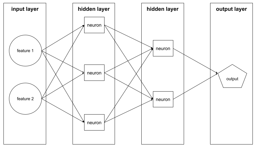
слой
A set of neurons in a neural network . Three common types of layers are as follows:
- The input layer , which provides values for all the features .
- One or more hidden layers , which find nonlinear relationships between the features and the label.
- The output layer , which provides the prediction.
For example, the following illustration shows a neural network with one input layer, two hidden layers, and one output layer:
In TensorFlow , layers are also Python functions that take Tensors and configuration options as input and produce other tensors as output.
скорость обучения
A floating-point number that tells the gradient descent algorithm how strongly to adjust weights and biases on each iteration . For example, a learning rate of 0.3 would adjust weights and biases three times more powerfully than a learning rate of 0.1.
Learning rate is a key hyperparameter . If you set the learning rate too low, training will take too long. If you set the learning rate too high, gradient descent often has trouble reaching convergence .
See Linear regression: Hyperparameters in Machine Learning Crash Course for more information.
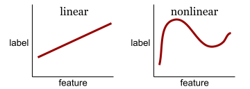
линейный
A relationship between two or more variables that can be represented solely through addition and multiplication.
The plot of a linear relationship is a line.
Contrast with nonlinear .
линейная модель
A model that assigns one weight per feature to make predictions . (Linear models also incorporate a bias .) In contrast, the relationship of features to predictions in deep models is generally nonlinear .
Linear models are usually easier to train and more interpretable than deep models. However, deep models can learn complex relationships between features.
Linear regression and logistic regression are two types of linear models.
линейная регрессия
A type of machine learning model in which both of the following are true:
- The model is a linear model .
- The prediction is a floating-point value. (This is the regression part of linear regression .)
Contrast linear regression with logistic regression . Also, contrast regression with classification .
See Linear regression in Machine Learning Crash Course for more information.
логистическая регрессия
A type of regression model that predicts a probability. Logistic regression models have the following characteristics:
- The label is categorical . The term logistic regression usually refers to binary logistic regression , that is, to a model that calculates probabilities for labels with two possible values. A less common variant, multinomial logistic regression , calculates probabilities for labels with more than two possible values.
- The loss function during training is Log Loss . (Multiple Log Loss units can be placed in parallel for labels with more than two possible values.)
- The model has a linear architecture, not a deep neural network. However, the remainder of this definition also applies to deep models that predict probabilities for categorical labels.
For example, consider a logistic regression model that calculates the probability of an input email being either spam or not spam. During inference, suppose the model predicts 0.72. Therefore, the model is estimating:
- A 72% chance of the email being spam.
- A 28% chance of the email not being spam.
A logistic regression model uses the following two-step architecture:
- The model generates a raw prediction (y') by applying a linear function of input features.
- The model uses that raw prediction as input to a sigmoid function , which converts the raw prediction to a value between 0 and 1, exclusive.
Like any regression model, a logistic regression model predicts a number. However, this number typically becomes part of a binary classification model as follows:
- If the predicted number is greater than the classification threshold , the binary classification model predicts the positive class.
- If the predicted number is less than the classification threshold, the binary classification model predicts the negative class.
See Logistic regression in Machine Learning Crash Course for more information.
Потери логарифма
The loss function used in binary logistic regression .
See Logistic regression: Loss and regularization in Machine Learning Crash Course for more information.
log-odds
The logarithm of the odds of some event.
потеря
During the training of a supervised model , a measure of how far a model's prediction is from its label .
A loss function calculates the loss.
See Linear regression: Loss in Machine Learning Crash Course for more information.
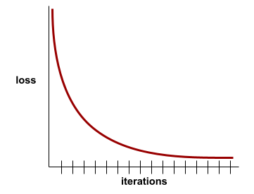
loss curve
A plot of loss as a function of the number of training iterations . The following plot shows a typical loss curve:

Loss curves can help you determine when your model is converging or overfitting .
Loss curves can plot all of the following types of loss:
See also generalization curve .
See Overfitting: Interpreting loss curves in Machine Learning Crash Course for more information.
функция потерь
During training or testing, a mathematical function that calculates the loss on a batch of examples. A loss function returns a lower loss for models that makes good predictions than for models that make bad predictions.
The goal of training is typically to minimize the loss that a loss function returns.
Many different kinds of loss functions exist. Pick the appropriate loss function for the kind of model you are building. For example:
- L 2 loss (or Mean Squared Error ) is the loss function for linear regression .
- Log Loss is the loss function for logistic regression .
М
машинное обучение
A program or system that trains a model from input data. The trained model can make useful predictions from new (never-before-seen) data drawn from the same distribution as the one used to train the model.
Machine learning also refers to the field of study concerned with these programs or systems.
See the Introduction to Machine Learning course for more information.
большинство класса
The more common label in a class-imbalanced dataset . For example, given a dataset containing 99% negative labels and 1% positive labels, the negative labels are the majority class.
Contrast with minority class .
See Datasets: Imbalanced datasets in Machine Learning Crash Course for more information.
mini-batch
A small, randomly selected subset of a batch processed in one iteration . The batch size of a mini-batch is usually between 10 and 1,000 examples.
For example, suppose the entire training set (the full batch) consists of 1,000 examples. Further suppose that you set the batch size of each mini-batch to 20. Therefore, each iteration determines the loss on a random 20 of the 1,000 examples and then adjusts the weights and biases accordingly.
It is much more efficient to calculate the loss on a mini-batch than the loss on all the examples in the full batch.
See Linear regression: Hyperparameters in Machine Learning Crash Course for more information.
класс меньшинства
The less common label in a class-imbalanced dataset . For example, given a dataset containing 99% negative labels and 1% positive labels, the positive labels are the minority class.
Contrast with majority class .
See Datasets: Imbalanced datasets in Machine Learning Crash Course for more information.
модель
In general, any mathematical construct that processes input data and returns output. Phrased differently, a model is the set of parameters and structure needed for a system to make predictions. In supervised machine learning , a model takes an example as input and infers a prediction as output. Within supervised machine learning, models differ somewhat. For example:
- A linear regression model consists of a set of weights and a bias .
- A neural network model consists of:
- A set of hidden layers , each containing one or more neurons .
- The weights and bias associated with each neuron.
- A decision tree model consists of:
- The shape of the tree; that is, the pattern in which the conditions and leaves are connected.
- The conditions and leaves.
You can save, restore, or make copies of a model.
Unsupervised machine learning also generates models, typically a function that can map an input example to the most appropriate cluster .
multi-class classification
In supervised learning, a classification problem in which the dataset contains more than two classes of labels. For example, the labels in the Iris dataset must be one of the following three classes:
- Ирис сетоза
- Iris virginica
- Iris versicolor
A model trained on the Iris dataset that predicts Iris type on new examples is performing multi-class classification.
In contrast, classification problems that distinguish between exactly two classes are binary classification models . For example, an email model that predicts either spam or not spam is a binary classification model.
In clustering problems, multi-class classification refers to more than two clusters.
See Neural networks: Multi-class classification in Machine Learning Crash Course for more information.
Н
negative class
In binary classification , one class is termed positive and the other is termed negative . The positive class is the thing or event that the model is testing for and the negative class is the other possibility. For example:
- The negative class in a medical test might be "not tumor."
- The negative class in an email classification model might be "not spam."
Contrast with positive class .
нейронная сеть
A model containing at least one hidden layer . A deep neural network is a type of neural network containing more than one hidden layer. For example, the following diagram shows a deep neural network containing two hidden layers.
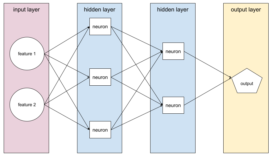
Each neuron in a neural network connects to all of the nodes in the next layer. For example, in the preceding diagram, notice that each of the three neurons in the first hidden layer separately connect to both of the two neurons in the second hidden layer.
Neural networks implemented on computers are sometimes called artificial neural networks to differentiate them from neural networks found in brains and other nervous systems.
Some neural networks can mimic extremely complex nonlinear relationships between different features and the label.
See also convolutional neural network and recurrent neural network .
See Neural networks in Machine Learning Crash Course for more information.
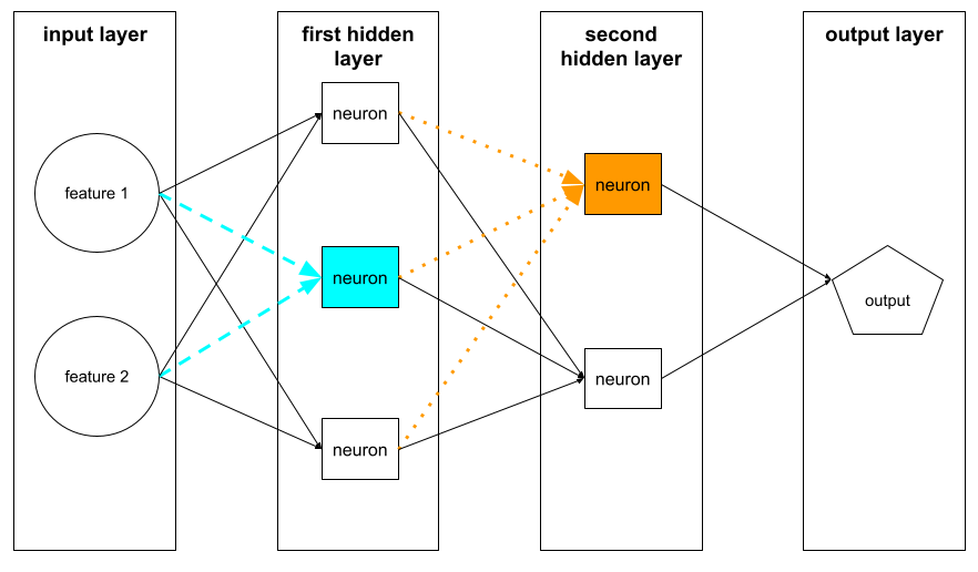
нейрон
In machine learning, a distinct unit within a hidden layer of a neural network . Each neuron performs the following two-step action:
- Calculates the weighted sum of input values multiplied by their corresponding weights.
- Passes the weighted sum as input to an activation function .
A neuron in the first hidden layer accepts inputs from the feature values in the input layer . A neuron in any hidden layer beyond the first accepts inputs from the neurons in the preceding hidden layer. For example, a neuron in the second hidden layer accepts inputs from the neurons in the first hidden layer.
The following illustration highlights two neurons and their inputs.
A neuron in a neural network mimics the behavior of neurons in brains and other parts of nervous systems.
node (neural network)
A neuron in a hidden layer .
See Neural Networks in Machine Learning Crash Course for more information.
nonlinear
A relationship between two or more variables that can't be represented solely through addition and multiplication. A linear relationship can be represented as a line; a nonlinear relationship can't be represented as a line. For example, consider two models that each relate a single feature to a single label. The model on the left is linear and the model on the right is nonlinear:
See Neural networks: Nodes and hidden layers in Machine Learning Crash Course to experiment with different kinds of nonlinear functions.
нестационарность
A feature whose values change across one or more dimensions, usually time. For example, consider the following examples of nonstationarity:
- The number of swimsuits sold at a particular store varies with the season.
- The quantity of a particular fruit harvested in a particular region is zero for much of the year but large for a brief period.
- Due to climate change, annual mean temperatures are shifting.
Contrast with stationarity .
нормализация
Broadly speaking, the process of converting a variable's actual range of values into a standard range of values, such as:
- от -1 до +1
- от 0 до 1
- Z-scores (roughly, -3 to +3)
For example, suppose the actual range of values of a certain feature is 800 to 2,400. As part of feature engineering , you could normalize the actual values down to a standard range, such as -1 to +1.
Normalization is a common task in feature engineering . Models usually train faster (and produce better predictions) when every numerical feature in the feature vector has roughly the same range.
See also Z-score normalization .
See Numerical Data: Normalization in Machine Learning Crash Course for more information.
numerical data
Features represented as integers or real-valued numbers. For example, a house valuation model would probably represent the size of a house (in square feet or square meters) as numerical data. Representing a feature as numerical data indicates that the feature's values have a mathematical relationship to the label. That is, the number of square meters in a house probably has some mathematical relationship to the value of the house.
Not all integer data should be represented as numerical data. For example, postal codes in some parts of the world are integers; however, integer postal codes shouldn't be represented as numerical data in models. That's because a postal code of 20000 is not twice (or half) as potent as a postal code of 10000. Furthermore, although different postal codes do correlate to different real estate values, we can't assume that real estate values at postal code 20000 are twice as valuable as real estate values at postal code 10000. Postal codes should be represented as categorical data instead.
Numerical features are sometimes called continuous features .
See Working with numerical data in Machine Learning Crash Course for more information.
О
офлайн
Synonym for static .
offline inference
The process of a model generating a batch of predictions and then caching (saving) those predictions. Apps can then access the inferred prediction from the cache rather than rerunning the model.
For example, consider a model that generates local weather forecasts (predictions) once every four hours. After each model run, the system caches all the local weather forecasts. Weather apps retrieve the forecasts from the cache.
Offline inference is also called static inference .
Contrast with online inference . See Production ML systems: Static versus dynamic inference in Machine Learning Crash Course for more information.
однократное кодирование
Representing categorical data as a vector in which:
- One element is set to 1.
- All other elements are set to 0.
One-hot encoding is commonly used to represent strings or identifiers that have a finite set of possible values. For example, suppose a certain categorical feature named Scandinavia has five possible values:
- "Дания"
- "Швеция"
- "Норвегия"
- "Финляндия"
- "Исландия"
One-hot encoding could represent each of the five values as follows:
| Страна | Вектор | ||||
|---|---|---|---|---|---|
| "Дания" | 1 | 0 | 0 | 0 | 0 |
| "Швеция" | 0 | 1 | 0 | 0 | 0 |
| "Норвегия" | 0 | 0 | 1 | 0 | 0 |
| "Финляндия" | 0 | 0 | 0 | 1 | 0 |
| "Исландия" | 0 | 0 | 0 | 0 | 1 |
Thanks to one-hot encoding, a model can learn different connections based on each of the five countries.
Representing a feature as numerical data is an alternative to one-hot encoding. Unfortunately, representing the Scandinavian countries numerically is not a good choice. For example, consider the following numeric representation:
- "Denmark" is 0
- "Sweden" is 1
- "Norway" is 2
- "Finland" is 3
- "Iceland" is 4
With numeric encoding, a model would interpret the raw numbers mathematically and would try to train on those numbers. However, Iceland isn't actually twice as much (or half as much) of something as Norway, so the model would come to some strange conclusions.
See Categorical data: Vocabulary and one-hot encoding in Machine Learning Crash Course for more information.
one-vs.-all
Given a classification problem with N classes, a solution consisting of N separate binary classification model—one binary classification model for each possible outcome. For example, given a model that classifies examples as animal, vegetable, or mineral, a one-vs.-all solution would provide the following three separate binary classification models:
- animal versus not animal
- vegetable versus not vegetable
- mineral versus not mineral
онлайн
Synonym for dynamic .
онлайн-вывод
Generating predictions on demand. For example, suppose an app passes input to a model and issues a request for a prediction. A system using online inference responds to the request by running the model (and returning the prediction to the app).
Contrast with offline inference .
See Production ML systems: Static versus dynamic inference in Machine Learning Crash Course for more information.
выходной слой
The "final" layer of a neural network. The output layer contains the prediction.
The following illustration shows a small deep neural network with an input layer, two hidden layers, and an output layer:
переобучение
Creating a model that matches the training data so closely that the model fails to make correct predictions on new data.
Regularization can reduce overfitting. Training on a large and diverse training set can also reduce overfitting.
See Overfitting in Machine Learning Crash Course for more information.
П
панды
A column-oriented data analysis API built on top of numpy . Many machine learning frameworks, including TensorFlow, support pandas data structures as inputs. See the pandas documentation for details.
параметр
The weights and biases that a model learns during training . For example, in a linear regression model, the parameters consist of the bias ( b ) and all the weights ( w 1 , w 2 , and so on) in the following formula:
In contrast, hyperparameters are the values that you (or a hyperparameter tuning service) supply to the model. For example, learning rate is a hyperparameter.
positive class
The class you are testing for.
For example, the positive class in a cancer model might be "tumor." The positive class in an email classification model might be "spam."
Contrast with negative class .
постобработка
Adjusting the output of a model after the model has been run. Post-processing can be used to enforce fairness constraints without modifying models themselves.
For example, one might apply post-processing to a binary classification model by setting a classification threshold such that equality of opportunity is maintained for some attribute by checking that the true positive rate is the same for all values of that attribute.
точность
A metric for classification models that answers the following question:
When the model predicted the positive class , what percentage of the predictions were correct?
Вот формула:
где:
- true positive means the model correctly predicted the positive class.
- false positive means the model mistakenly predicted the positive class.
For example, suppose a model made 200 positive predictions. Of these 200 positive predictions:
- 150 were true positives.
- 50 were false positives.
В этом случае:
Contrast with accuracy and recall .
See Classification: Accuracy, recall, precision and related metrics in Machine Learning Crash Course for more information.
прогноз
A model's output. For example:
- The prediction of a binary classification model is either the positive class or the negative class.
- The prediction of a multi-class classification model is one class.
- The prediction of a linear regression model is a number.
proxy labels
Data used to approximate labels not directly available in a dataset.
For example, suppose you must train a model to predict employee stress level. Your dataset contains a lot of predictive features but doesn't contain a label named stress level. Undaunted, you pick "workplace accidents" as a proxy label for stress level. After all, employees under high stress get into more accidents than calm employees. Or do they? Maybe workplace accidents actually rise and fall for multiple reasons.
As a second example, suppose you want is it raining? to be a Boolean label for your dataset, but your dataset doesn't contain rain data. If photographs are available, you might establish pictures of people carrying umbrellas as a proxy label for is it raining? Is that a good proxy label? Possibly, but people in some cultures may be more likely to carry umbrellas to protect against sun than the rain.
Proxy labels are often imperfect. When possible, choose actual labels over proxy labels. That said, when an actual label is absent, pick the proxy label very carefully, choosing the least horrible proxy label candidate.
See Datasets: Labels in Machine Learning Crash Course for more information.
Р
ТРЯПКА
Abbreviation for retrieval-augmented generation .
оценщик
A human who provides labels for examples . "Annotator" is another name for rater.
See Categorical data: Common issues in Machine Learning Crash Course for more information.
отзывать
A metric for classification models that answers the following question:
When ground truth was the positive class , what percentage of predictions did the model correctly identify as the positive class?
Вот формула:
\[\text{Recall} = \frac{\text{true positives}} {\text{true positives} + \text{false negatives}} \]
где:
- true positive means the model correctly predicted the positive class.
- false negative means that the model mistakenly predicted the negative class .
For instance, suppose your model made 200 predictions on examples for which ground truth was the positive class. Of these 200 predictions:
- 180 were true positives.
- 20 were false negatives.
В этом случае:
\[\text{Recall} = \frac{\text{180}} {\text{180} + \text{20}} = 0.9 \]
See Classification: Accuracy, recall, precision and related metrics for more information.
Выпрямленная линейная функция активации (ReLU)
An activation function with the following behavior:
- If input is negative or zero, then the output is 0.
- If input is positive, then the output is equal to the input.
Например:
- If the input is -3, then the output is 0.
- If the input is +3, then the output is 3.0.
Here is a plot of ReLU:
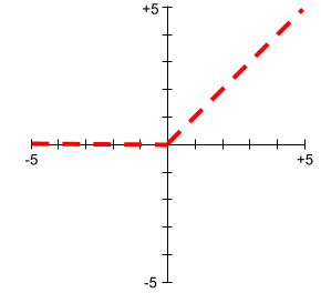
ReLU is a very popular activation function. Despite its simple behavior, ReLU still enables a neural network to learn nonlinear relationships between features and the label .
регрессионная модель
Informally, a model that generates a numerical prediction. (In contrast, a classification model generates a class prediction.) For example, the following are all regression models:
- A model that predicts a certain house's value in Euros, such as 423,000.
- A model that predicts a certain tree's life expectancy in years, such as 23.2.
- A model that predicts the amount of rain in inches that will fall in a certain city over the next six hours, such as 0.18.
Two common types of regression models are:
- Linear regression , which finds the line that best fits label values to features.
- Logistic regression , which generates a probability between 0.0 and 1.0 that a system typically then maps to a class prediction.
Not every model that outputs numerical predictions is a regression model. In some cases, a numeric prediction is really just a classification model that happens to have numeric class names. For example, a model that predicts a numeric postal code is a classification model, not a regression model.
регуляризация
Any mechanism that reduces overfitting . Popular types of regularization include:
- L 1 regularization
- L 2 regularization
- dropout regularization
- early stopping (this is not a formal regularization method, but can effectively limit overfitting)
Regularization can also be defined as the penalty on a model's complexity.
See Overfitting: Model complexity in Machine Learning Crash Course for more information.
regularization rate
A number that specifies the relative importance of regularization during training. Raising the regularization rate reduces overfitting but may reduce the model's predictive power. Conversely, reducing or omitting the regularization rate increases overfitting.
See Overfitting: L2 regularization in Machine Learning Crash Course for more information.
РеЛУ
Abbreviation for Rectified Linear Unit .
retrieval-augmented generation (RAG)
A technique for improving the quality of large language model (LLM) output by grounding it with sources of knowledge retrieved after the model was trained. RAG improves the accuracy of LLM responses by providing the trained LLM with access to information retrieved from trusted knowledge bases or documents.
Common motivations to use retrieval-augmented generation include:
- Increasing the factual accuracy of a model's generated responses.
- Giving the model access to knowledge it was not trained on.
- Changing the knowledge that the model uses.
- Enabling the model to cite sources.
For example, suppose that a chemistry app uses the PaLM API to generate summaries related to user queries. When the app's backend receives a query, the backend:
- Searches for ("retrieves") data that's relevant to the user's query.
- Appends ("augments") the relevant chemistry data to the user's query.
- Instructs the LLM to create a summary based on the appended data.
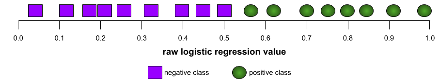
ROC (receiver operating characteristic) Curve
A graph of true positive rate versus false positive rate for different classification thresholds in binary classification.
The shape of an ROC curve suggests a binary classification model's ability to separate positive classes from negative classes. Suppose, for example, that a binary classification model perfectly separates all the negative classes from all the positive classes:
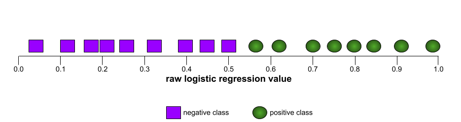
The ROC curve for the preceding model looks as follows:
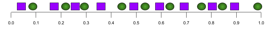
In contrast, the following illustration graphs the raw logistic regression values for a terrible model that can't separate negative classes from positive classes at all:
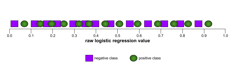
The ROC curve for this model looks as follows:
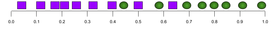
Meanwhile, back in the real world, most binary classification models separate positive and negative classes to some degree, but usually not perfectly. So, a typical ROC curve falls somewhere between the two extremes:
The point on an ROC curve closest to (0.0,1.0) theoretically identifies the ideal classification threshold. However, several other real-world issues influence the selection of the ideal classification threshold. For example, perhaps false negatives cause far more pain than false positives.
A numerical metric called AUC summarizes the ROC curve into a single floating-point value.
Среднеквадратичная ошибка (RMSE)
The square root of the Mean Squared Error .
С
сигмоидная функция
A mathematical function that "squishes" an input value into a constrained range, typically 0 to 1 or -1 to +1. That is, you can pass any number (two, a million, negative billion, whatever) to a sigmoid and the output will still be in the constrained range. A plot of the sigmoid activation function looks as follows:
The sigmoid function has several uses in machine learning, including:
- Converting the raw output of a logistic regression or multinomial regression model to a probability.
- Acting as an activation function in some neural networks.
софтмакс
A function that determines probabilities for each possible class in a multi-class classification model . The probabilities add up to exactly 1.0. For example, the following table shows how softmax distributes various probabilities:
| Image is a... | Вероятность |
|---|---|
| собака | .85 |
| кот | .13 |
| лошадь | .02 |
Softmax is also called full softmax .
Contrast with candidate sampling .
See Neural networks: Multi-class classification in Machine Learning Crash Course for more information.
sparse feature
A feature whose values are predominately zero or empty. For example, a feature containing a single 1 value and a million 0 values is sparse. In contrast, a dense feature has values that are predominantly not zero or empty.
In machine learning, a surprising number of features are sparse features. Categorical features are usually sparse features. For example, of the 300 possible tree species in a forest, a single example might identify just a maple tree . Or, of the millions of possible videos in a video library, a single example might identify just "Casablanca."
In a model, you typically represent sparse features with one-hot encoding . If the one-hot encoding is big, you might put an embedding layer on top of the one-hot encoding for greater efficiency.
sparse representation
Storing only the position(s) of nonzero elements in a sparse feature.
For example, suppose a categorical feature named species identifies the 36 tree species in a particular forest. Further assume that each example identifies only a single species.
You could use a one-hot vector to represent the tree species in each example. A one-hot vector would contain a single 1 (to represent the particular tree species in that example) and 35 0 s (to represent the 35 tree species not in that example). So, the one-hot representation of maple might look something like the following:
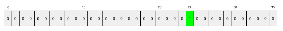
Alternatively, sparse representation would simply identify the position of the particular species. If maple is at position 24, then the sparse representation of maple would simply be:
24
Notice that the sparse representation is much more compact than the one-hot representation.
Click the icon for a slightly more complex example.
Suppose each example in your model must represent the words—but not the order of those words—in an English sentence. English consists of about 170,000 words, so English is a categorical feature with about 170,000 elements. Most English sentences use an extremely tiny fraction of those 170,000 words, so the set of words in a single example is almost certainly going to be sparse data.
Consider the following sentence:
My dog is a great dog
You could use a variant of one-hot vector to represent the words in this sentence. In this variant, multiple cells in the vector can contain a nonzero value. Furthermore, in this variant, a cell can contain an integer other than one. Although the words "my", "is", "a", and "great" appear only once in the sentence, the word "dog" appears twice. Using this variant of one-hot vectors to represent the words in this sentence yields the following 170,000-element vector:
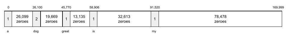
A sparse representation of the same sentence would simply be:
0: 1
26100: 2
45770: 1
58906: 1
91520: 1
See Working with categorical data in Machine Learning Crash Course for more information.
разреженный вектор
A vector whose values are mostly zeroes. See also sparse feature and sparsity .
squared loss
Synonym for L 2 loss .
статический
Something done once rather than continuously. The terms static and offline are synonyms. The following are common uses of static and offline in machine learning:
- static model (or offline model ) is a model trained once and then used for a while.
- static training (or offline training ) is the process of training a static model.
- static inference (or offline inference ) is a process in which a model generates a batch of predictions at a time.
Contrast with dynamic .
static inference
Synonym for offline inference .
stationarity
A feature whose values don't change across one or more dimensions, usually time. For example, a feature whose values look about the same in 2021 and 2023 exhibits stationarity.
In the real world, very few features exhibit stationarity. Even features synonymous with stability (like sea level) change over time.
Contrast with nonstationarity .
stochastic gradient descent (SGD)
A gradient descent algorithm in which the batch size is one. In other words, SGD trains on a single example chosen uniformly at random from a training set .
See Linear regression: Hyperparameters in Machine Learning Crash Course for more information.
контролируемое машинное обучение
Training a model from features and their corresponding labels . Supervised machine learning is analogous to learning a subject by studying a set of questions and their corresponding answers. After mastering the mapping between questions and answers, a student can then provide answers to new (never-before-seen) questions on the same topic.
Compare with unsupervised machine learning .
See Supervised Learning in the Introduction to ML course for more information.
synthetic feature
A feature not present among the input features, but assembled from one or more of them. Methods for creating synthetic features include the following:
- Bucketing a continuous feature into range bins.
- Creating a feature cross .
- Multiplying (or dividing) one feature value by other feature value(s) or by itself. For example, if
aandbare input features, then the following are examples of synthetic features:- аб
- а 2
- Applying a transcendental function to a feature value. For example, if
cis an input feature, then the following are examples of synthetic features:- sin(c)
- ln(c)
Features created by normalizing or scaling alone are not considered synthetic features.
Т
тест потери
A metric representing a model's loss against the test set . When building a model , you typically try to minimize test loss. That's because a low test loss is a stronger quality signal than a low training loss or low validation loss .
A large gap between test loss and training loss or validation loss sometimes suggests that you need to increase the regularization rate .
обучение
The process of determining the ideal parameters (weights and biases) comprising a model . During training, a system reads in examples and gradually adjusts parameters. Training uses each example anywhere from a few times to billions of times.
See Supervised Learning in the Introduction to ML course for more information.
потери в обучении
A metric representing a model's loss during a particular training iteration. For example, suppose the loss function is Mean Squared Error . Perhaps the training loss (the Mean Squared Error) for the 10th iteration is 2.2, and the training loss for the 100th iteration is 1.9.
A loss curve plots training loss versus the number of iterations. A loss curve provides the following hints about training:
- A downward slope implies that the model is improving.
- An upward slope implies that the model is getting worse.
- A flat slope implies that the model has reached convergence .
For example, the following somewhat idealized loss curve shows:
- A steep downward slope during the initial iterations, which implies rapid model improvement.
- A gradually flattening (but still downward) slope until close to the end of training, which implies continued model improvement at a somewhat slower pace then during the initial iterations.
- A flat slope towards the end of training, which suggests convergence.
Although training loss is important, see also generalization .
training-serving skew
The difference between a model's performance during training and that same model's performance during serving .
тренировочный набор
The subset of the dataset used to train a model .
Traditionally, examples in the dataset are divided into the following three distinct subsets:
- a training set
- a validation set
- a test set
Ideally, each example in the dataset should belong to only one of the preceding subsets. For example, a single example shouldn't belong to both the training set and the validation set.
See Datasets: Dividing the original dataset in Machine Learning Crash Course for more information.
true negative (TN)
An example in which the model correctly predicts the negative class . For example, the model infers that a particular email message is not spam , and that email message really is not spam .
true positive (TP)
An example in which the model correctly predicts the positive class . For example, the model infers that a particular email message is spam, and that email message really is spam.
true positive rate (TPR)
Synonym for recall . That is:
True positive rate is the y-axis in an ROC curve .
У
несоответствие
Producing a model with poor predictive ability because the model hasn't fully captured the complexity of the training data. Many problems can cause underfitting, including:
- Training on the wrong set of features .
- Training for too few epochs or at too low a learning rate .
- Training with too high a regularization rate .
- Providing too few hidden layers in a deep neural network.
See Overfitting in Machine Learning Crash Course for more information.
unlabeled example
An example that contains features but no label . For example, the following table shows three unlabeled examples from a house valuation model, each with three features but no house value:
| Количество спален | Количество ванных комнат | House age |
|---|---|---|
| 3 | 2 | 15 |
| 2 | 1 | 72 |
| 4 | 2 | 34 |
In supervised machine learning , models train on labeled examples and make predictions on unlabeled examples .
In semi-supervised and unsupervised learning, unlabeled examples are used during training.
Contrast unlabeled example with labeled example .
машинное обучение без учителя
Training a model to find patterns in a dataset, typically an unlabeled dataset.
The most common use of unsupervised machine learning is to cluster data into groups of similar examples. For example, an unsupervised machine learning algorithm can cluster songs based on various properties of the music. The resulting clusters can become an input to other machine learning algorithms (for example, to a music recommendation service). Clustering can help when useful labels are scarce or absent. For example, in domains such as anti-abuse and fraud, clusters can help humans better understand the data.
Contrast with supervised machine learning .
See What is Machine Learning? in the Introduction to ML course for more information.
В
валидация
The initial evaluation of a model's quality. Validation checks the quality of a model's predictions against the validation set .
Because the validation set differs from the training set , validation helps guard against overfitting .
You might think of evaluating the model against the validation set as the first round of testing and evaluating the model against the test set as the second round of testing.
потери валидации
A metric representing a model's loss on the validation set during a particular iteration of training.
See also generalization curve .
набор валидации
The subset of the dataset that performs initial evaluation against a trained model . Typically, you evaluate the trained model against the validation set several times before evaluating the model against the test set .
Traditionally, you divide the examples in the dataset into the following three distinct subsets:
- a training set
- a validation set
- a test set
Ideally, each example in the dataset should belong to only one of the preceding subsets. For example, a single example shouldn't belong to both the training set and the validation set.
See Datasets: Dividing the original dataset in Machine Learning Crash Course for more information.
В
масса
A value that a model multiplies by another value. Training is the process of determining a model's ideal weights; inference is the process of using those learned weights to make predictions.
See Linear regression in Machine Learning Crash Course for more information.
взвешенная сумма
The sum of all the relevant input values multiplied by their corresponding weights. For example, suppose the relevant inputs consist of the following:
| входное значение | входной вес |
| 2 | -1.3 |
| -1 | 0,6 |
| 3 | 0,4 |
The weighted sum is therefore:
weighted sum = (2)(-1.3) + (-1)(0.6) + (3)(0.4) = -2.0
A weighted sum is the input argument to an activation function .
З
Z-score normalization
A scaling technique that replaces a raw feature value with a floating-point value representing the number of standard deviations from that feature's mean. For example, consider a feature whose mean is 800 and whose standard deviation is 100. The following table shows how Z-score normalization would map the raw value to its Z-score:
| Сырое значение | Z-показатель |
|---|---|
| 800 | 0 |
| 950 | +1.5 |
| 575 | -2.25 |
The machine learning model then trains on the Z-scores for that feature instead of on the raw values.
See Numerical data: Normalization in Machine Learning Crash Course for more information.