Dynamic World V1

데이터 세트 제공: 2015-06-27T00:00:00Z–2026-03-24T15:32:08.527000Z
데이터 세트 출처: World Resources Institute Google

태그: global google landcover landuse landuse-landcover nrt sentinel2-derived

설명

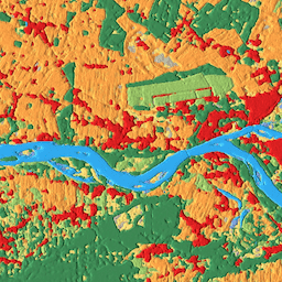
Dynamic World는 9개 클래스의 클래스 확률 및 라벨 정보를 포함하는 10m 실시간에 가까운 (NRT) 토지 이용/토지 피복 (LULC) 데이터 세트입니다.

Dynamic World 예측은 2015-06-27부터 현재까지 Sentinel-2 L1C 컬렉션에 사용할 수 있습니다. Sentinel-2의 재방문 빈도는 위도에 따라 2~5일입니다. Dynamic World 예측은 CLOUDY_PIXEL_PERCENTAGE <= 35%인 Sentinel-2 L1C 이미지에 대해 생성됩니다. 예측은 S2 Cloud Probability, Cloud Displacement Index, Directional Distance Transform의 조합을 사용하여 구름과 구름 그림자를 삭제하도록 마스크 처리됩니다.

Dynamic World 컬렉션의 이미지는 파생된 개별 Sentinel-2 L1C 애셋 이름과 일치하는 이름을 갖습니다. 예를 들면 다음과 같습니다.

ee.Image('COPERNICUS/S2/20160711T084022_20160711T084751_T35PKT')

ee.Image('GOOGLE/DYNAMICWORLD/V1/20160711T084022_20160711T084751_T35PKT')라는 이름의 일치하는 Dynamic World 이미지가 있습니다.

'label' 대역을 제외한 모든 확률 대역의 합은 1입니다.

Dynamic World 데이터 세트에 대해 자세히 알아보고 합성 생성, 지역 통계 계산, 시계열 작업의 예를 보려면 Dynamic World 소개 튜토리얼 시리즈를 참고하세요.

Dynamic World 클래스 추정치는 작은 이동 창의 공간 컨텍스트를 사용하여 단일 이미지에서 파생되므로 작물과 같이 시간이 지남에 따라 피복으로 부분적으로 정의되는 예측된 토지 피복의 상위 1개 '확률'은 명확한 구별 기능이 없는 경우 비교적 낮을 수 있습니다. 건조한 기후의 고수익 표면, 모래, 태양 반사 등도 이 현상을 나타낼 수 있습니다.

Dynamic World 클래스에 확실히 속하는 픽셀만 선택하려면 상위 1개 예측의 추정된 '확률'을 임곗값 처리하여 Dynamic World 출력을 마스크 처리하는 것이 좋습니다.

대역

픽셀 크기: 10m (모든 대역)

이름	최대	픽셀 크기	설명
`water`	1	10미터	물로 완전히 피복될 예상 확률
`trees`	1	10미터	나무로 완전히 피복될 예상 확률
`grass`	1	10미터	잔디로 완전히 피복될 예상 확률
`flooded_vegetation`	1	10미터	침수된 초목으로 완전히 피복될 예상 확률
`crops`	1	10미터	작물로 완전히 피복될 예상 확률
`shrub_and_scrub`	1	10미터	관목과 수풀로 완전히 피복될 예상 확률
`built`	1	10미터	빌드됨으로 완전히 피복될 예상 확률
`bare`	1	10미터	노출됨으로 완전히 피복될 예상 확률
`snow_and_ice`	1	10미터	눈과 얼음으로 완전히 피복될 예상 확률
`label`	8	10미터	예상 확률이 가장 높은 대역의 색인

라벨 클래스 표

값	색상	설명
0	#419bdf	물
1	#397d49	나무
2	#88b053	잔디
3	#7a87c6	flooded_vegetation
4	#e49635	작물
5	#dfc35a	shrub_and_scrub
6	#c4281b	빌드됨
7	#a59b8f	노출됨
8	#b39fe1	snow_and_ice

이미지 속성

이미지 속성

이름	유형	설명
dynamicworld_algorithm_version	STRING	이미지를 생성하는 데 사용된 Dynamic World 모델 및 추론 프로세스를 고유하게 식별하는 버전 문자열입니다.
qa_algorithm_version	STRING	이미지를 생성하는 데 사용된 클라우드 마스크 처리 프로세스를 고유하게 식별하는 버전 문자열입니다.

이용약관

이용약관

이 데이터 세트는 CC-BY 4.0에 따라 라이선스가 부여되며 다음과 같은 저작자 표시가 필요합니다. '이 데이터 세트는 National Geographic Society 및 World Resources Institute와 제휴하여 Google에서 Dynamic World 프로젝트를 위해 제작했습니다.'

수정된 Copernicus Sentinel 데이터[2015년~현재]를 포함합니다. Sentinel 데이터 법적 고지를 참고하세요.

인용

Brown, C.F., Brumby, S.P., Guzder-Williams, B. 외. Dynamic World, 실시간에 가까운 전 세계 10m 토지 이용 토지 피복 매핑. Sci Data 9, 251 (2022). doi:10.1038/s41597-022-01307-4

DOI

https://doi.org/10.1038/s41597-022-01307-4

Earth Engine으로 탐색

코드 편집기 (JavaScript)

// Construct a collection of corresponding Dynamic World and Sentinel-2 for
// inspection. Filter by region and date.
var START = ee.Date('2021-04-02');
var END = START.advance(1, 'day');

var colFilter = ee.Filter.and(
    ee.Filter.bounds(ee.Geometry.Point(20.6729, 52.4305)),
    ee.Filter.date(START, END));

var dwCol = ee.ImageCollection('GOOGLE/DYNAMICWORLD/V1').filter(colFilter);
var s2Col = ee.ImageCollection('COPERNICUS/S2_HARMONIZED');

// Link DW and S2 source images.
var linkedCol = dwCol.linkCollection(s2Col, s2Col.first().bandNames());

// Get example DW image with linked S2 image.
var linkedImg = ee.Image(linkedCol.first());

// Create a visualization that blends DW class label with probability.
// Define list pairs of DW LULC label and color.
var CLASS_NAMES = [
    'water', 'trees', 'grass', 'flooded_vegetation', 'crops',
    'shrub_and_scrub', 'built', 'bare', 'snow_and_ice'];

var VIS_PALETTE = [
    '419bdf', '397d49', '88b053', '7a87c6', 'e49635', 'dfc35a', 'c4281b',
    'a59b8f', 'b39fe1'];

// Create an RGB image of the label (most likely class) on [0, 1].
var dwRgb = linkedImg
    .select('label')
    .visualize({min: 0, max: 8, palette: VIS_PALETTE})
    .divide(255);

// Get the most likely class probability.
var top1Prob = linkedImg.select(CLASS_NAMES).reduce(ee.Reducer.max());

// Create a hillshade of the most likely class probability on [0, 1];
var top1ProbHillshade =
    ee.Terrain.hillshade(top1Prob.multiply(100))
    .divide(255);

// Combine the RGB image with the hillshade.
var dwRgbHillshade = dwRgb.multiply(top1ProbHillshade);

// Display the Dynamic World visualization with the source Sentinel-2 image.
Map.setCenter(20.6729, 52.4305, 12);
Map.addLayer(
    linkedImg, {min: 0, max: 3000, bands: ['B4', 'B3', 'B2']}, 'Sentinel-2 L1C');
Map.addLayer(
    dwRgbHillshade, {min: 0, max: 0.65}, 'Dynamic World V1 - label hillshade');

Python 설정

Python API 및 대화형 개발을 위한 geemap 사용에 관한 자세한 내용은 Python 환경 페이지를 참고하세요.

import ee
import geemap.core as geemap

Colab(Python)

# Construct a collection of corresponding Dynamic World and Sentinel-2 for
# inspection. Filter by region and date.
START = ee.Date('2021-04-02')
END = START.advance(1, 'day')

col_filter = ee.Filter.And(
    ee.Filter.bounds(ee.Geometry.Point(20.6729, 52.4305)),
    ee.Filter.date(START, END),
)

dw_col = ee.ImageCollection('GOOGLE/DYNAMICWORLD/V1').filter(col_filter)
s2_col = ee.ImageCollection('COPERNICUS/S2_HARMONIZED');

# Link DW and S2 source images.
linked_col = dw_col.linkCollection(s2_col, s2_col.first().bandNames());

# Get example DW image with linked S2 image.
linked_image = ee.Image(linked_col.first())

# Create a visualization that blends DW class label with probability.
# Define list pairs of DW LULC label and color.
CLASS_NAMES = [
    'water',
    'trees',
    'grass',
    'flooded_vegetation',
    'crops',
    'shrub_and_scrub',
    'built',
    'bare',
    'snow_and_ice',
]

VIS_PALETTE = [
    '419bdf',
    '397d49',
    '88b053',
    '7a87c6',
    'e49635',
    'dfc35a',
    'c4281b',
    'a59b8f',
    'b39fe1',
]

# Create an RGB image of the label (most likely class) on [0, 1].
dw_rgb = (
    linked_image.select('label')
    .visualize(min=0, max=8, palette=VIS_PALETTE)
    .divide(255)
)

# Get the most likely class probability.
top1_prob = linked_image.select(CLASS_NAMES).reduce(ee.Reducer.max())

# Create a hillshade of the most likely class probability on [0, 1]
top1_prob_hillshade = ee.Terrain.hillshade(top1_prob.multiply(100)).divide(255)

# Combine the RGB image with the hillshade.
dw_rgb_hillshade = dw_rgb.multiply(top1_prob_hillshade)

# Display the Dynamic World visualization with the source Sentinel-2 image.
m = geemap.Map()
m.set_center(20.6729, 52.4305, 12)
m.add_layer(
    linked_image,
    {'min': 0, 'max': 3000, 'bands': ['B4', 'B3', 'B2']},
    'Sentinel-2 L1C',
)
m.add_layer(
    dw_rgb_hillshade,
    {'min': 0, 'max': 0.65},
    'Dynamic World V1 - label hillshade',
)
m

코드 편집기에서 열기

Dynamic World V1

Dynamic World는 9개 클래스의 클래스 확률 및 라벨 정보를 포함하는 10m 실시간에 가까운 (NRT) 토지 이용/토지 피복 (LULC) 데이터 세트입니다. Dynamic World 예측은 2015-06-27부터 현재까지 Sentinel-2 L1C 컬렉션에 사용할 수 있습니다. Sentinel-2의 재방문 빈도는 위도에 따라 2~5일입니다. Dynamic World …

GOOGLE/DYNAMICWORLD/V1, global,google,landcover,landuse,landuse-landcover,nrt,sentinel2-derived

2015-06-27T00:00:00Z/2026-03-24T15:32:08.527000Z

-90 -180 90 180

Google Earth Engine

https://developers.google.com/earth-engine/datasets

Dynamic World V1 컬렉션을 사용해 정리하기 내 환경설정을 기준으로 콘텐츠를 저장하고 분류하세요.

설명

대역

이미지 속성

이용약관

인용

DOI

Earth Engine으로 탐색

코드 편집기 (JavaScript)

Colab(Python)

Dynamic World V1