Page Summary
-
PIF matching is a relative radiometric normalization technique used to harmonize radiometric differences between images acquired under varying conditions or times.
-
The process involves identifying pseudo-invariant features (areas with minimal spectral change) between images.
-
Spectral distance metrics, like spectral information divergence (SID), are used to automatically identify these pseudo-invariant features.
-
A linear transformation is applied to the entire image based on the spectral differences found within the identified pseudo-invariant features to achieve radiometric normalization.
-
This technique allows for more accurate comparisons and change detection between multi-temporal images.
Background
Relative radiometric normalization techniques like histogram matching, multivariate alteration detection (MAD), and PIF matching apply transformations between images that were acquired at different times, under different conditions, or by different sensors, reducing radiometric differences to allow for more accurate comparisons and change detection (Schroeder et al., 2006). PIF matching works by identifying areas with minimal spectral change between images, known as pseudo-invariant features, and applying a linear transformation to the entire image based on the spectral differences between these areas.
Input Data
The code below loads two Planet SkySat images acquired before and after a
logging operation in Peru, clips them to a small area of interest, selects the
relevant multispectral bands, and uses the
register
method to correct a slight misregistration between images.
var aoi = ee.Geometry.Point([-75.0608, -8.2736]).buffer(3000).bounds();
var bands = ee.List(['N', 'R', 'G', 'B']);

var before = ee.Image('SKYSAT/GEN-A/PUBLIC/ORTHO/MULTISPECTRAL/s02_20150804T151429Z')
  .select(bands)
  .clip(aoi);
var after = ee.Image('SKYSAT/GEN-A/PUBLIC/ORTHO/MULTISPECTRAL/s01_20150910T154218Z')
  .select(bands)
  .clip(aoi)
  .register(before, 100);
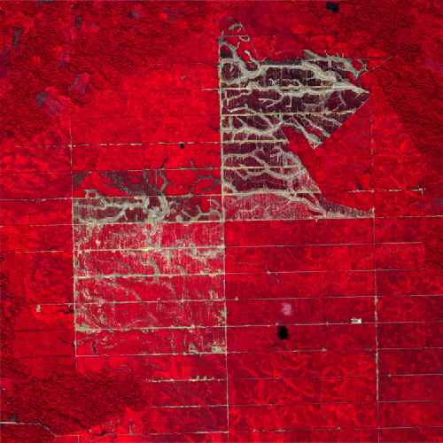
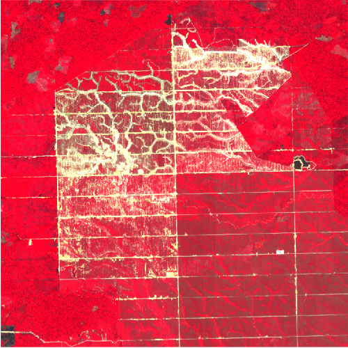
Adding the images to the map shows the radiometric mismatch between them: the 'after' image appears much brighter than the 'before' image, making direct comparisons more difficult.
Map.centerObject(aoi);
Map.addLayer(before, {min: 1000, max: 5000}, 'Before');
Map.addLayer(after, {min: 1000, max: 5000}, 'After');
| Before | After |
|---|---|
 |
 |
Identifying Pseudo-Invariant Features
With the before and after images loaded and aligned, the next step is to identify spectrally stable, pseudo-invariant features that can be used to match the images. While PIFs can be selected manually by identifying unchanged areas and digitizing points or polygons around them, this approach can be time-consuming and subjective. Spectral distance metrics provide an automated method for measuring similarity between pixels, which can then be used to select a subset of pixels with the smallest spectral changes.
Measuring Spectral Distance
The code below uses the spectralDistance
method to calculate spectral information divergence (SID) between the before
and after images. You can also experiment with other distance metrics like
spectral angle mapper (SAM) or squared euclidean distance (SED) to see how
they affect results.
var distance = before.spectralDistance(after, 'SID');
Map.addLayer(distance, {min: 0, max: 0.4}, 'Spectral distance');
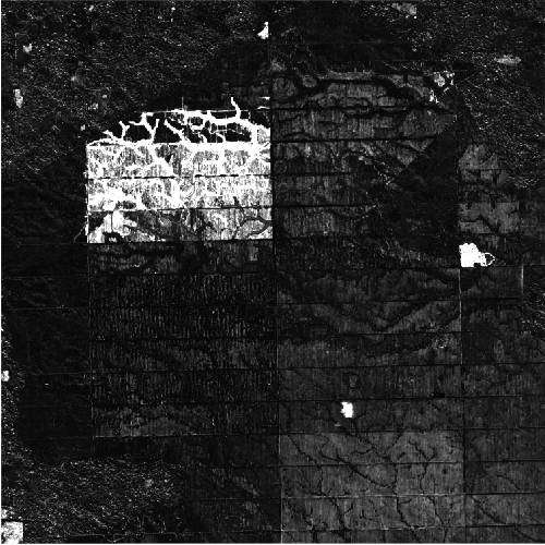
Visualizing spectral distance highlights areas of change that correspond with logging, road construction, and cloud shadows:
Selecting Stable Pixels
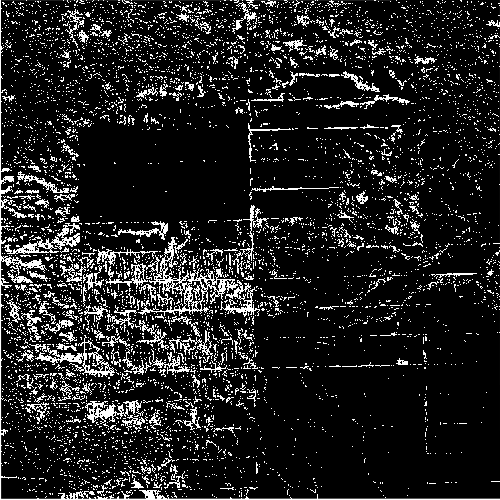
The next step is to select a subset of pixels that experienced little or no change. This can be done by applying a percentile reducer over the area of interest to identify a spectral distance threshold, then selecting pixels with distances below that threshold. The code below uses a 10th percentile threshold, but you may want to modify the percentile to see how it affects results. Higher percentiles will select pixels with greater spectral distances, allowing transformations to normalize larger radiometric differences at the risk of introducing bias from outlying pixels.
var threshold = distance.reduceRegion({
  reducer: ee.Reducer.percentile([10]),
  geometry: aoi,
  scale: 1,
  bestEffort: true,
  maxPixels: 1e6,
}).getNumber('distance');

var pif = distance.lt(threshold);
Map.addLayer(pif, {}, 'PIF mask');
Applying the Transformation
With pseudo-invariant pixels identified, the next step is to build linear transformations between these areas in the before and after image, which can then be applied to the entire image. This can be done by mapping over each band and:
- Masking the before and after image to the PIF.
- Using a
linearFitreducer to calculate regression coefficients between the masked images in the area of interest. - Applying the linear coefficients to match the after image to the before image.
The function below applies all three steps to a single band for convenience:
function matchBand(band) {
  var beforePif = before.select([band]).updateMask(pif);
  var afterPif = after.select([band]).updateMask(pif);

  var args = {
    reducer: ee.Reducer.linearFit(),
    geometry: aoi,
    scale: 1,
    maxPixels: 1e6,
    bestEffort: true
  };

  var coeffs = ee.Image.cat([afterPif, beforePif])
    .reduceRegion(args);

  return after
    .select([band])
    .multiply(coeffs.getNumber('scale'))
    .add(coeffs.getNumber('offset'));
}
Mapping that function over the list of bands defined at the beginning of
the tutorial will return a list of matched single-band images, which can then
be combined back into a multi-band image.
var matchedBands = bands.map(matchBand);
var matched = ee.ImageCollection(matchedBands).toBands().rename(bands);
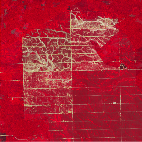
Here are the results, showing the before, after (matched), and after (original) images:
Map.addLayer(before, {min: 1000, max: 5000}, 'Before');
Map.addLayer(matched, {min: 1000, max: 5000}, 'After (Matched)');
Map.addLayer(after, {min: 1000, max: 5000}, 'After (Original)');
| Before | After (Matched) | After (Original) |
|---|---|---|
 |
 |
 |
Conclusion
The full code is below, or you can open it in the Code Editor.
// Select an area of interest and define multispectral bands to use
var aoi = ee.Geometry.Point([-75.0608, -8.2736]).buffer(3000).bounds();
var bands = ee.List(['N', 'R', 'G', 'B']);

// Select a pair of Planet SkySat images acquired before and after deforestation
var before = ee.Image('SKYSAT/GEN-A/PUBLIC/ORTHO/MULTISPECTRAL/s02_20150804T151429Z')
  .select(bands)
  .clip(aoi);
var after = ee.Image('SKYSAT/GEN-A/PUBLIC/ORTHO/MULTISPECTRAL/s01_20150910T154218Z')
  .select(bands)
  .clip(aoi)
  .register(before, 100);

// Calculate spectral distance as a measure of change between the images
var distance = before.spectralDistance(after, 'sid');

// Identify the 10th percentile of change
var threshold = distance.reduceRegion({
  reducer: ee.Reducer.percentile([10]),
  geometry: aoi,
  scale: 1,
  bestEffort: true,
  maxPixels: 1e6,
}).getNumber('distance');

// Define pseudo-invariant features below the change threshold
var pif = distance.lt(threshold);

function matchBand(band) {
  // Select just the PIF areas in each image
  var beforePif = before.select([band]).updateMask(pif);
  var afterPif = after.select([band]).updateMask(pif);

  // Define a linear reducer to calculate a transformation between images
  var args = {
    reducer: ee.Reducer.linearFit(),
    geometry: aoi,
    scale: 1,
    maxPixels: 1e6,
    bestEffort: true
    };

  // Calculate the linear coefficients
  var coeffs = ee.Image.cat([afterPif, beforePif])
    .reduceRegion(args);

  // Apply the coefficients to match the after band to the before band
  return after
    .select([band])
    .multiply(coeffs.getNumber('scale'))
    .add(coeffs.getNumber('offset'));
}

// Match each band, then combine them back into a single multi-band image
var matchedBands = bands.map(matchBand);
var matched = ee.ImageCollection(matchedBands).toBands().rename(bands);

Map.centerObject(aoi);
Map.addLayer(distance, {min: 0, max: 0.4}, 'Spectral distance');
Map.addLayer(pif, {}, 'PIF mask');
Map.addLayer(before, {min: 1000, max: 5000}, 'Before');
Map.addLayer(matched, {min: 1000, max: 5000}, 'After (Matched)');
Map.addLayer(after, {min: 1000, max: 5000}, 'After (Original)');