
Les sections suivantes présentent un exemple de problème MIP et expliquent comment le résoudre. Voici le problème:
Maximisez la x + 10y sous réserve des contraintes suivantes:
x + 7y≤ 17,5- 0 ≤
x≤ 3,5 - 0 ≤
y x,yentiers
Étant donné que les contraintes sont linéaires, il ne s'agit que d'un problème d'optimisation linéaire, dans lequel les solutions doivent être des entiers. Le graphique ci-dessous indique des points entiers dans la région réalisable pour le problème.
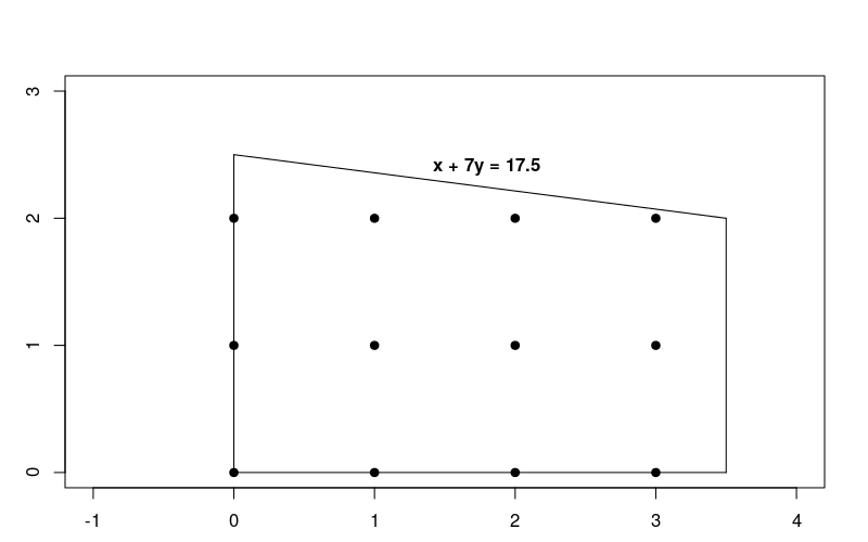
Notez que ce problème est très semblable à celui d'optimisation linéaire décrit dans la section Résoudre un problème lié à la page de destination, mais que les solutions doivent être des entiers.
Étapes de base pour résoudre un problème MIP
Pour résoudre un problème MIP, votre programme doit inclure les étapes suivantes:
- Importer le wrapper de solution linéaire
- déclarer le résolveur MIP,
- définir les variables,
- définir les contraintes,
- définir l'objectif,
- à appeler le résolveur MIP
- afficher la solution
Solution utilisant le MPSolver
La section suivante présente un programme qui résout le problème à l'aide du wrapper MPSolver et d'un résolveur MIP.
Le résolveur MIP OR-Tools est défini par défaut sur SCIP.
Importer le wrapper de solution linéaire
Importez (ou incluez) le wrapper de solution linéaire OR-Tools, une interface pour les résolveurs MIP et les résolveurs linéaires, comme indiqué ci-dessous.
Python
from ortools.linear_solver import pywraplp
C++
#include <memory>

#include "ortools/linear_solver/linear_solver.h"
Java
import com.google.ortools.Loader;
import com.google.ortools.linearsolver.MPConstraint;
import com.google.ortools.linearsolver.MPObjective;
import com.google.ortools.linearsolver.MPSolver;
import com.google.ortools.linearsolver.MPVariable;
C#
using System;
using Google.OrTools.LinearSolver;
Déclarer le résolveur MIP
Le code suivant déclare le résolveur MIP du problème. Cet exemple utilise le résolveur tiers SCIP.
Python
# Create the mip solver with the SCIP backend.
solver = pywraplp.Solver.CreateSolver("SAT")
if not solver:
    return
C++
// Create the mip solver with the SCIP backend.
std::unique_ptr<MPSolver> solver(MPSolver::CreateSolver("SCIP"));
if (!solver) {
  LOG(WARNING) << "SCIP solver unavailable.";
  return;
}
Java
// Create the linear solver with the SCIP backend.
MPSolver solver = MPSolver.createSolver("SCIP");
if (solver == null) {
  System.out.println("Could not create solver SCIP");
  return;
}
C#
// Create the linear solver with the SCIP backend.
Solver solver = Solver.CreateSolver("SCIP");
if (solver is null)
{
    return;
}
Définir les variables
Le code suivant définit les variables du problème.
Python
infinity = solver.infinity()
# x and y are integer non-negative variables.
x = solver.IntVar(0.0, infinity, "x")
y = solver.IntVar(0.0, infinity, "y")

print("Number of variables =", solver.NumVariables())
C++
const double infinity = solver->infinity();
// x and y are integer non-negative variables.
MPVariable* const x = solver->MakeIntVar(0.0, infinity, "x");
MPVariable* const y = solver->MakeIntVar(0.0, infinity, "y");

LOG(INFO) << "Number of variables = " << solver->NumVariables();
Java
double infinity = java.lang.Double.POSITIVE_INFINITY;
// x and y are integer non-negative variables.
MPVariable x = solver.makeIntVar(0.0, infinity, "x");
MPVariable y = solver.makeIntVar(0.0, infinity, "y");

System.out.println("Number of variables = " + solver.numVariables());
C#
// x and y are integer non-negative variables.
Variable x = solver.MakeIntVar(0.0, double.PositiveInfinity, "x");
Variable y = solver.MakeIntVar(0.0, double.PositiveInfinity, "y");

Console.WriteLine("Number of variables = " + solver.NumVariables());
Le programme utilise la méthode MakeIntVar (ou une variante, selon le langage de codage) pour créer les variables x et y qui acceptent des valeurs entières non négatives.
Définir les contraintes
Le code suivant définit les contraintes du problème.
Python
# x + 7 * y <= 17.5.
solver.Add(x + 7 * y <= 17.5)

# x <= 3.5.
solver.Add(x <= 3.5)

print("Number of constraints =", solver.NumConstraints())
C++
// x + 7 * y <= 17.5.
MPConstraint* const c0 = solver->MakeRowConstraint(-infinity, 17.5, "c0");
c0->SetCoefficient(x, 1);
c0->SetCoefficient(y, 7);

// x <= 3.5.
MPConstraint* const c1 = solver->MakeRowConstraint(-infinity, 3.5, "c1");
c1->SetCoefficient(x, 1);
c1->SetCoefficient(y, 0);

LOG(INFO) << "Number of constraints = " << solver->NumConstraints();
Java
// x + 7 * y <= 17.5.
MPConstraint c0 = solver.makeConstraint(-infinity, 17.5, "c0");
c0.setCoefficient(x, 1);
c0.setCoefficient(y, 7);

// x <= 3.5.
MPConstraint c1 = solver.makeConstraint(-infinity, 3.5, "c1");
c1.setCoefficient(x, 1);
c1.setCoefficient(y, 0);

System.out.println("Number of constraints = " + solver.numConstraints());
C#
// x + 7 * y <= 17.5.
solver.Add(x + 7 * y <= 17.5);

// x <= 3.5.
solver.Add(x <= 3.5);

Console.WriteLine("Number of constraints = " + solver.NumConstraints());
Définir l’objectif
Le code suivant définit objective function pour le problème.
Python
# Maximize x + 10 * y.
solver.Maximize(x + 10 * y)
C++
// Maximize x + 10 * y.
MPObjective* const objective = solver->MutableObjective();
objective->SetCoefficient(x, 1);
objective->SetCoefficient(y, 10);
objective->SetMaximization();
Java
// Maximize x + 10 * y.
MPObjective objective = solver.objective();
objective.setCoefficient(x, 1);
objective.setCoefficient(y, 10);
objective.setMaximization();
C#
// Maximize x + 10 * y.
solver.Maximize(x + 10 * y);
Appeler le résolveur
Le code suivant appelle le résolveur.
Python
print(f"Solving with {solver.SolverVersion()}")
status = solver.Solve()
C++
const MPSolver::ResultStatus result_status = solver->Solve();
// Check that the problem has an optimal solution.
if (result_status != MPSolver::OPTIMAL) {
  LOG(FATAL) << "The problem does not have an optimal solution!";
}
Java
final MPSolver.ResultStatus resultStatus = solver.solve();
C#
Solver.ResultStatus resultStatus = solver.Solve();
Afficher la solution
Le code suivant affiche la solution.
Python
if status == pywraplp.Solver.OPTIMAL:
    print("Solution:")
    print("Objective value =", solver.Objective().Value())
    print("x =", x.solution_value())
    print("y =", y.solution_value())
else:
    print("The problem does not have an optimal solution.")
C++
LOG(INFO) << "Solution:";
LOG(INFO) << "Objective value = " << objective->Value();
LOG(INFO) << "x = " << x->solution_value();
LOG(INFO) << "y = " << y->solution_value();
Java
if (resultStatus == MPSolver.ResultStatus.OPTIMAL) {
  System.out.println("Solution:");
  System.out.println("Objective value = " + objective.value());
  System.out.println("x = " + x.solutionValue());
  System.out.println("y = " + y.solutionValue());
} else {
  System.err.println("The problem does not have an optimal solution!");
}
C#
// Check that the problem has an optimal solution.
if (resultStatus != Solver.ResultStatus.OPTIMAL)
{
    Console.WriteLine("The problem does not have an optimal solution!");
    return;
}
Console.WriteLine("Solution:");
Console.WriteLine("Objective value = " + solver.Objective().Value());
Console.WriteLine("x = " + x.SolutionValue());
Console.WriteLine("y = " + y.SolutionValue());
Voici la solution à ce problème.
Number of variables = 2
Number of constraints = 2
Solution:
Objective value = 23
x = 3
y = 2
La valeur optimale de la fonction d'objectif est de 23, ce qui se produit au point x = 3, y = 2.
Terminer les programmes
Voici les programmes complets.
Python
from ortools.linear_solver import pywraplp


def main():
    # Create the mip solver with the SCIP backend.
    solver = pywraplp.Solver.CreateSolver("SAT")
    if not solver:
        return

    infinity = solver.infinity()
    # x and y are integer non-negative variables.
    x = solver.IntVar(0.0, infinity, "x")
    y = solver.IntVar(0.0, infinity, "y")

    print("Number of variables =", solver.NumVariables())

    # x + 7 * y <= 17.5.
    solver.Add(x + 7 * y <= 17.5)

    # x <= 3.5.
    solver.Add(x <= 3.5)

    print("Number of constraints =", solver.NumConstraints())

    # Maximize x + 10 * y.
    solver.Maximize(x + 10 * y)

    print(f"Solving with {solver.SolverVersion()}")
    status = solver.Solve()

    if status == pywraplp.Solver.OPTIMAL:
        print("Solution:")
        print("Objective value =", solver.Objective().Value())
        print("x =", x.solution_value())
        print("y =", y.solution_value())
    else:
        print("The problem does not have an optimal solution.")

    print("\nAdvanced usage:")
    print(f"Problem solved in {solver.wall_time():d} milliseconds")
    print(f"Problem solved in {solver.iterations():d} iterations")
    print(f"Problem solved in {solver.nodes():d} branch-and-bound nodes")


if __name__ == "__main__":
    main()
C++
#include <memory>

#include "ortools/linear_solver/linear_solver.h"

namespace operations_research {
void SimpleMipProgram() {
  // Create the mip solver with the SCIP backend.
  std::unique_ptr<MPSolver> solver(MPSolver::CreateSolver("SCIP"));
  if (!solver) {
    LOG(WARNING) << "SCIP solver unavailable.";
    return;
  }

  const double infinity = solver->infinity();
  // x and y are integer non-negative variables.
  MPVariable* const x = solver->MakeIntVar(0.0, infinity, "x");
  MPVariable* const y = solver->MakeIntVar(0.0, infinity, "y");

  LOG(INFO) << "Number of variables = " << solver->NumVariables();

  // x + 7 * y <= 17.5.
  MPConstraint* const c0 = solver->MakeRowConstraint(-infinity, 17.5, "c0");
  c0->SetCoefficient(x, 1);
  c0->SetCoefficient(y, 7);

  // x <= 3.5.
  MPConstraint* const c1 = solver->MakeRowConstraint(-infinity, 3.5, "c1");
  c1->SetCoefficient(x, 1);
  c1->SetCoefficient(y, 0);

  LOG(INFO) << "Number of constraints = " << solver->NumConstraints();

  // Maximize x + 10 * y.
  MPObjective* const objective = solver->MutableObjective();
  objective->SetCoefficient(x, 1);
  objective->SetCoefficient(y, 10);
  objective->SetMaximization();

  const MPSolver::ResultStatus result_status = solver->Solve();
  // Check that the problem has an optimal solution.
  if (result_status != MPSolver::OPTIMAL) {
    LOG(FATAL) << "The problem does not have an optimal solution!";
  }

  LOG(INFO) << "Solution:";
  LOG(INFO) << "Objective value = " << objective->Value();
  LOG(INFO) << "x = " << x->solution_value();
  LOG(INFO) << "y = " << y->solution_value();

  LOG(INFO) << "\nAdvanced usage:";
  LOG(INFO) << "Problem solved in " << solver->wall_time() << " milliseconds";
  LOG(INFO) << "Problem solved in " << solver->iterations() << " iterations";
  LOG(INFO) << "Problem solved in " << solver->nodes()
            << " branch-and-bound nodes";
}
}  // namespace operations_research

int main(int argc, char** argv) {
  operations_research::SimpleMipProgram();
  return EXIT_SUCCESS;
}
Java
package com.google.ortools.linearsolver.samples;
import com.google.ortools.Loader;
import com.google.ortools.linearsolver.MPConstraint;
import com.google.ortools.linearsolver.MPObjective;
import com.google.ortools.linearsolver.MPSolver;
import com.google.ortools.linearsolver.MPVariable;

/** Minimal Mixed Integer Programming example to showcase calling the solver. */
public final class SimpleMipProgram {
  public static void main(String[] args) {
    Loader.loadNativeLibraries();
    // Create the linear solver with the SCIP backend.
    MPSolver solver = MPSolver.createSolver("SCIP");
    if (solver == null) {
      System.out.println("Could not create solver SCIP");
      return;
    }

    double infinity = java.lang.Double.POSITIVE_INFINITY;
    // x and y are integer non-negative variables.
    MPVariable x = solver.makeIntVar(0.0, infinity, "x");
    MPVariable y = solver.makeIntVar(0.0, infinity, "y");

    System.out.println("Number of variables = " + solver.numVariables());

    // x + 7 * y <= 17.5.
    MPConstraint c0 = solver.makeConstraint(-infinity, 17.5, "c0");
    c0.setCoefficient(x, 1);
    c0.setCoefficient(y, 7);

    // x <= 3.5.
    MPConstraint c1 = solver.makeConstraint(-infinity, 3.5, "c1");
    c1.setCoefficient(x, 1);
    c1.setCoefficient(y, 0);

    System.out.println("Number of constraints = " + solver.numConstraints());

    // Maximize x + 10 * y.
    MPObjective objective = solver.objective();
    objective.setCoefficient(x, 1);
    objective.setCoefficient(y, 10);
    objective.setMaximization();

    final MPSolver.ResultStatus resultStatus = solver.solve();

    if (resultStatus == MPSolver.ResultStatus.OPTIMAL) {
      System.out.println("Solution:");
      System.out.println("Objective value = " + objective.value());
      System.out.println("x = " + x.solutionValue());
      System.out.println("y = " + y.solutionValue());
    } else {
      System.err.println("The problem does not have an optimal solution!");
    }

    System.out.println("\nAdvanced usage:");
    System.out.println("Problem solved in " + solver.wallTime() + " milliseconds");
    System.out.println("Problem solved in " + solver.iterations() + " iterations");
    System.out.println("Problem solved in " + solver.nodes() + " branch-and-bound nodes");
  }

  private SimpleMipProgram() {}
}
C#
using System;
using Google.OrTools.LinearSolver;

public class SimpleMipProgram
{
    static void Main()
    {
        // Create the linear solver with the SCIP backend.
        Solver solver = Solver.CreateSolver("SCIP");
        if (solver is null)
        {
            return;
        }

        // x and y are integer non-negative variables.
        Variable x = solver.MakeIntVar(0.0, double.PositiveInfinity, "x");
        Variable y = solver.MakeIntVar(0.0, double.PositiveInfinity, "y");

        Console.WriteLine("Number of variables = " + solver.NumVariables());

        // x + 7 * y <= 17.5.
        solver.Add(x + 7 * y <= 17.5);

        // x <= 3.5.
        solver.Add(x <= 3.5);

        Console.WriteLine("Number of constraints = " + solver.NumConstraints());

        // Maximize x + 10 * y.
        solver.Maximize(x + 10 * y);

        Solver.ResultStatus resultStatus = solver.Solve();

        // Check that the problem has an optimal solution.
        if (resultStatus != Solver.ResultStatus.OPTIMAL)
        {
            Console.WriteLine("The problem does not have an optimal solution!");
            return;
        }
        Console.WriteLine("Solution:");
        Console.WriteLine("Objective value = " + solver.Objective().Value());
        Console.WriteLine("x = " + x.SolutionValue());
        Console.WriteLine("y = " + y.SolutionValue());

        Console.WriteLine("\nAdvanced usage:");
        Console.WriteLine("Problem solved in " + solver.WallTime() + " milliseconds");
        Console.WriteLine("Problem solved in " + solver.Iterations() + " iterations");
        Console.WriteLine("Problem solved in " + solver.Nodes() + " branch-and-bound nodes");
    }
}
Comparer l'optimisation linéaire et l'optimisation entière
Comparons la solution au problème d'optimisation des entiers (illustrée ci-dessus) et celle au problème d'optimisation linéaire correspondant, dans lequel les contraintes d'entiers sont supprimées. Vous pouvez deviner que la solution au problème entier serait le point entier dans la région faisable la plus proche de la solution linéaire, à savoir le point x = 0, y = 2. Mais comme vous allez le voir
suivant, ce n'est pas le cas.
Vous pouvez facilement modifier le programme de la section précédente pour résoudre le problème linéaire en apportant les modifications suivantes:
- Remplacer le résolveur MIP
avec l'outil de résolution de pages de destination
Python
# Create the mip solver with the SCIP backend.
solver = pywraplp.Solver.CreateSolver("SAT")
if not solver:
    return
C++
// Create the mip solver with the SCIP backend.
std::unique_ptr<MPSolver> solver(MPSolver::CreateSolver("SCIP"));
if (!solver) {
  LOG(WARNING) << "SCIP solver unavailable.";
  return;
}
Java
// Create the linear solver with the SCIP backend.
MPSolver solver = MPSolver.createSolver("SCIP");
if (solver == null) {
  System.out.println("Could not create solver SCIP");
  return;
}
C#
// Create the linear solver with the SCIP backend. Solver solver = Solver.CreateSolver("SCIP"); if (solver is null) { return; }Python
# Create the linear solver with the GLOP backend.
solver = pywraplp.Solver.CreateSolver("GLOP")
if not solver:
    return
C++
// Create the linear solver with the GLOP backend.
std::unique_ptr<MPSolver> solver(MPSolver::CreateSolver("GLOP"));
Java
// Create the linear solver with the GLOP backend.
MPSolver solver = MPSolver.createSolver("GLOP");
if (solver == null) {
  System.out.println("Could not create solver SCIP");
  return;
}
C#
// Create the linear solver with the GLOP backend. Solver solver = Solver.CreateSolver("GLOP"); if (solver is null) { return; } - Remplacer les variables entières
avec des variables continues
Python
infinity = solver.infinity()
# x and y are integer non-negative variables.
x = solver.IntVar(0.0, infinity, "x")
y = solver.IntVar(0.0, infinity, "y")

print("Number of variables =", solver.NumVariables())
C++
const double infinity = solver->infinity();
// x and y are integer non-negative variables.
MPVariable* const x = solver->MakeIntVar(0.0, infinity, "x");
MPVariable* const y = solver->MakeIntVar(0.0, infinity, "y");

LOG(INFO) << "Number of variables = " << solver->NumVariables();
Java
double infinity = java.lang.Double.POSITIVE_INFINITY;
// x and y are integer non-negative variables.
MPVariable x = solver.makeIntVar(0.0, infinity, "x");
MPVariable y = solver.makeIntVar(0.0, infinity, "y");

System.out.println("Number of variables = " + solver.numVariables());
C#
// x and y are integer non-negative variables. Variable x = solver.MakeIntVar(0.0, double.PositiveInfinity, "x"); Variable y = solver.MakeIntVar(0.0, double.PositiveInfinity, "y"); Console.WriteLine("Number of variables = " + solver.NumVariables());Python
infinity = solver.infinity()
# Create the variables x and y.
x = solver.NumVar(0.0, infinity, "x")
y = solver.NumVar(0.0, infinity, "y")

print("Number of variables =", solver.NumVariables())
C++
const double infinity = solver->infinity();
// Create the variables x and y.
MPVariable* const x = solver->MakeNumVar(0.0, infinity, "x");
MPVariable* const y = solver->MakeNumVar(0.0, infinity, "y");

LOG(INFO) << "Number of variables = " << solver->NumVariables();
Java
double infinity = java.lang.Double.POSITIVE_INFINITY;
// Create the variables x and y.
MPVariable x = solver.makeNumVar(0.0, infinity, "x");
MPVariable y = solver.makeNumVar(0.0, infinity, "y");

System.out.println("Number of variables = " + solver.numVariables());
C#
// Create the variables x and y.
Variable x = solver.MakeNumVar(0.0, double.PositiveInfinity, "x");
Variable y = solver.MakeNumVar(0.0, double.PositiveInfinity, "y");

Console.WriteLine("Number of variables = " + solver.NumVariables());
Après avoir apporté ces modifications et exécuté à nouveau le programme, vous obtenez la sortie suivante:
Number of variables = 2
Number of constraints = 2
Objective value = 25.000000
x = 0.000000
y = 2.500000
La solution au problème linéaire se produit au point x = 0, y = 2.5, où la fonction objectif est égale à 25. Voici un graphique montrant les solutions aux
problèmes linéaires et entiers.
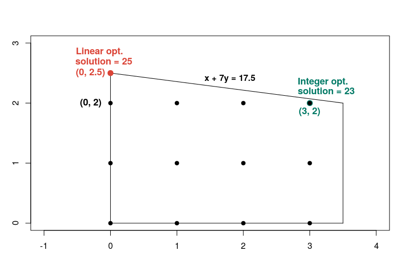
Notez que la solution entière n'est pas proche de la solution linéaire, par rapport à la plupart des autres points entiers dans la région réalisable. En général, les solutions à un problème d'optimisation linéaire et les problèmes d'optimisation des entiers correspondants peuvent être éloignés les uns des autres. Pour cette raison, ces deux types de problèmes nécessitent des méthodes différentes pour les résoudre.