# Advantages and disadvantages of k-means
K-means is useful and efficient in many machine learning contexts, but has
some distinct weaknesses.
## Advantages of k-means
Relatively simple to implement.
Scales to large data sets.
Always converges.
Allows warm-starting the positions of centroids.
Smoothly adapts to new examples.
Can be generalized to clusters of different shapes and sizes, such as elliptical clusters.
### Generalizing k-means
A straightforward implementation of k-means can struggle with clusters of
different densities and sizes. The left side of Figure 1 shows the clusters
we'd expect to see, while the right side shows the clusters proposed by k-means.
 **Figure 1: Ungeneralized k-means example.**
For better performance on imbalanced clusters like the ones shown in Figure 1,
you can generalize, that is, adapt, k-means. Figure 2 shows three different
datasets clustered with two different generalizations. The first dataset shows
k-means without generalization, while the second and third allow for clusters to
vary in width.
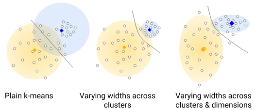 **Figure 2: k-means clustering with and without generalization.**
This course doesn't cover how to generalize k-means, but those interested
should see [Clustering -- k-means Gaussian mixture
models](http://www.cs.cmu.edu/%7Eguestrin/Class/10701-S07/Slides/clustering.pdf)
by Carlos Guestrin from Carnegie Mellon University.
## Disadvantages of k-means
\\(k\\) must be chosen manually.
Results depend on initial values.
For low \\(k\\), you can mitigate this dependence by running k-means several
times with different initial values and picking the best result. As \\(k\\)
increases, you need **k-means seeding** to pick better initial
centroids For a full discussion of k-means seeding, see
["A Comparative
Study of Efficient Initialization Methods for the K-means Clustering
Algorithm,"](https://arxiv.org/abs/1209.1960) by M. Emre Celebi, Hassan A. Kingravi, and Patricio A. Vela.
Difficulty clustering data of varying sizes and densities without generalization.
Difficulty clustering outliers.
Centroids can be dragged by outliers, or outliers might get their own cluster
instead of being ignored. Consider removing or clipping outliers before
clustering.
Difficulty scaling with number of dimensions.
As the number of dimensions in the data increases, a distance-based similarity
measure converges to a constant value between any given examples. Reduce
dimensionality either by using
[**PCA**](https://wikipedia.org/wiki/Principal_component_analysis)
on the feature data or by using **spectral clustering** to modify the clustering
algorithm.
### Curse of dimensionality and spectral clustering
In these three plots, notice how, as dimensions increase, the standard deviation
in distance between examples shrinks relative to the mean distance between
examples. This
convergence means that k-means becomes less effective at distinguishing between
examples as the dimensionality of the data increases. This is referred to as
the **curse of dimensionality**.
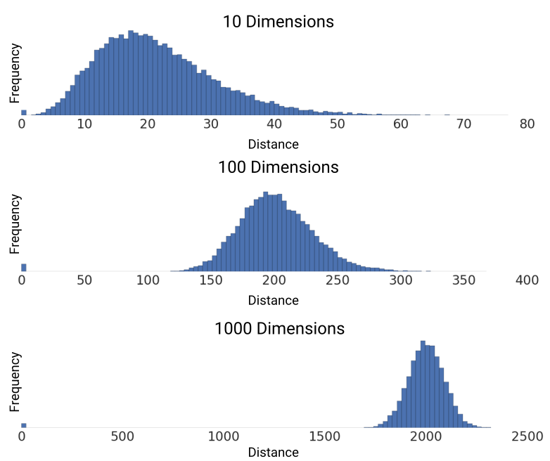 **Figure 3: A demonstration of the curse of dimensionality. Each plot shows the pairwise distances between 200 random points.**
You can avoid this diminishment in performance with **spectral clustering**,
which adds pre-clustering steps to the algorithm. To perform spectral
clustering:
1. Reduce the dimensionality of feature data by using PCA.
2. Project all data points into the lower-dimensional subspace.
3. Cluster the data in this subspace using your chosen algorithm.
See [*A Tutorial on Spectral
Clustering*](https://github.com/petermartigny/Advanced-Machine-Learning/blob/master/DataLab2/Luxburg07_tutorial_4488%5B0%5D.pdf) by Ulrike von Luxburg for more information on spectral
clustering.
> [!IMPORTANT]
> **Key terms:**
>
>
>
> - spectral clustering
>
>
>