Interpret Results and Adjust Clustering

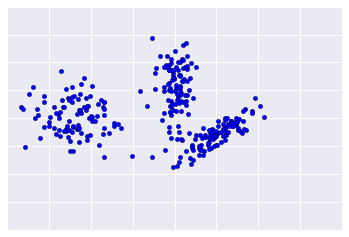
Because clustering is unsupervised, no “truth” is available to verify results. The absence of truth complicates assessing quality. Further, real-world datasets typically do not fall into obvious clusters of examples like the dataset shown in Figure 1.

Figure 1: An ideal data plot; real-world data rarely looks like this.

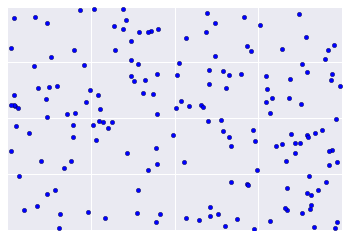
Sadly, real-world data looks more like Figure 2, making it difficult to visually assess clustering quality.

Figure 2: A true-to-life data plot

The flowchart below summarizes how to check the quality of your clustering. We'll expand upon the summary in the following sections.

Click here to see a larger version of this chart.

Step One: Quality of Clustering

Checking the quality of clustering is not a rigorous process because clustering lacks “truth”. Here are guidelines that you can iteratively apply to improve the quality of your clustering.

First, perform a visual check that the clusters look as expected, and that examples that you consider similar do appear in the same cluster. Then check these commonly-used metrics as described in the following sections:

• Cluster cardinality
• Cluster magnitude
• Performance of downstream system

Note: While several other metrics exist to evaluate clustering quality, these three metrics are commonly-used and beneficial.

Figure 2: Cardinality of several clusters.

Cluster cardinality

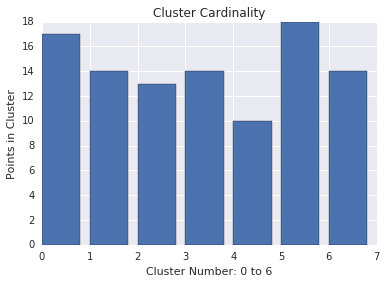
Cluster cardinality is the number of examples per cluster. Plot the cluster cardinality for all clusters and investigate clusters that are major outliers. For example, in Figure 2, investigate cluster number 5.

Figure 3: Magnitude of several clusters.

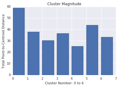
Cluster magnitude

Cluster magnitude is the sum of distances from all examples to the centroid of the cluster. Similar to cardinality, check how the magnitude varies across the clusters, and investigate anomalies. For example, in Figure 3, investigate cluster number 0.

Figure 4: Cardinality vs. Magnitude of several clusters.

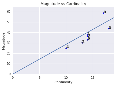
Magnitude vs. Cardinality

Notice that a higher cluster cardinality tends to result in a higher cluster magnitude, which intuitively makes sense. Clusters are anomalous when cardinality doesn't correlate with magnitude relative to the other clusters. Find anomalous clusters by plotting magnitude against cardinality. For example, in Figure 4, fitting a line to the cluster metrics shows that cluster number 0 is anomalous.

Performance of Downstream System

Since clustering output is often used in downstream ML systems, check if the downstream system’s performance improves when your clustering process changes. The impact on your downstream performance provides a real-world test for the quality of your clustering. The disadvantage is that this check is complex to perform.

Questions to Investigate If Problems are Found

If you find problems, then check your data preparation and similarity measure, asking yourself the following questions:

• Is your data scaled?
• Is your similarity measure correct?
• Is your algorithm performing semantically meaningful operations on the data?
• Do your algorithm’s assumptions match the data?

Step Two: Performance of the Similarity Measure

Your clustering algorithm is only as good as your similarity measure. Make sure your similarity measure returns sensible results. The simplest check is to identify pairs of examples that are known to be more or less similar than other pairs. Then, calculate the similarity measure for each pair of examples. Ensure that the similarity measure for more similar examples is higher than the similarity measure for less similar examples.

The examples you use to spot check your similarity measure should be representative of the data set. Ensure that your similarity measure holds for all your examples. Careful verification ensures that your similarity measure, whether manual or supervised, is consistent across your dataset. If your similarity measure is inconsistent for some examples, then those examples will not be clustered with similar examples.

If you find examples with inaccurate similarities, then your similarity measure probably does not capture the feature data that distinguishes those examples. Experiment with your similarity measure and determine whether you get more accurate similarities.

Step Three: Optimum Number of Clusters

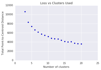
k-means requires you to decide the number of clusters \(k\) beforehand. How do you determine the optimal value of \(k\)? Try running the algorithm for increasing \(k\) and note the sum of cluster magnitudes. As \(k\) increases, clusters become smaller, and the total distance decreases. Plot this distance against the number of clusters.

As shown in Figure 4, at a certain \(k\), the reduction in loss becomes marginal with increasing \(k\). Mathematically, that's roughly the \(k\) where the slope crosses above -1 (\(\theta > 135^{\circ}\)). This guideline doesn't pinpoint an exact value for the optimum \(k\) but only an approximate value. For the plot shown, the optimum \(k\) is approximately 11. If you prefer more granular clusters, then you can choose a higher \(k\) using this plot as guidance.

Figure 4: Loss vs. number of clusters