Author(s): [mortcanty](https://github.com/mortcanty "View the profile for mortcanty on GitHub") Tutorials contributed by the Earth Engine developer community are not part of the official Earth Engine product documentation.
|---|---|
| [ Run in Google Colab](https://colab.research.google.com/github/google/earthengine-community/blob/master/tutorials/imad-tutorial-pt2/index.ipynb) | [ View source on GitHub](https://github.com/google/earthengine-community/blob/master/tutorials/imad-tutorial-pt2/index.ipynb) |
## Context
In Part 1 of this tutorial, a statistical approach to detecting changes in pairs of
multispectral remote sensing images, called Multivariate Alteration Detection (MAD), was
explained. The MAD change images were obtained by first maximizing the correlations
between the original image bands and then subtracting one from the other. The resulting
difference bands, called MAD variates, contained the change information. They were shown
to be ordered by increasing variance and to be mutually uncorrelated. However, they were
also seen to be not easily interpretable.
Now, in Part 2, we introduce an iteration scheme that performs the MAD transformation
exclusively on those pixels that mark areas in the images which have not physically
changed. This establishes a well-defined background of invariant pixels against which
to discriminate changes.
## Preliminaries
This tutorial will optionally export assets. Edit the following
`EXPORT_PATH` variable to specify the location to store the assets.
All assets that are needed to complete the tutorial are hosted by Earth Engine,
but if you'd like to display assets that you export, replace paths as needed.
# Enter your own export to assets path name here ---
EXPORT_PATH = 'projects/YOUR_GEE_PROJECT_NAME/assets/imad/'
# ---
import ee
ee.Authenticate(auth_mode='notebook')
ee.Initialize()
# Import other packages used in the tutorial
%matplotlib inline
import geemap
import numpy as np
import random, time
import matplotlib.pyplot as plt
from scipy.stats import norm, chi2
from pprint import pprint # for pretty printing
### Routines from Part 1
def trunc(values, dec = 3):
'''Truncate a 1-D array to dec decimal places.'''
return np.trunc(values*10**dec)/(10**dec)
# Display an image in a one percent linear stretch.
def display_ls(image, map, name, centered = False):
bns = image.bandNames().length().getInfo()
if bns == 3:
image = image.rename('B1', 'B2', 'B3')
pb_99 = ['B1_p99', 'B2_p99', 'B3_p99']
pb_1 = ['B1_p1', 'B2_p1', 'B3_p1']
img = ee.Image.rgb(image.select('B1'), image.select('B2'), image.select('B3'))
else:
image = image.rename('B1')
pb_99 = ['B1_p99']
pb_1 = ['B1_p1']
img = image.select('B1')
percentiles = image.reduceRegion(ee.Reducer.percentile([1, 99]), maxPixels=1e11)
mx = percentiles.values(pb_99)
if centered:
mn = ee.Array(mx).multiply(-1).toList()
else:
mn = percentiles.values(pb_1)
map.addLayer(img, {'min': mn, 'max': mx}, name)
def collect(aoi, t1a ,t1b, t2a, t2b):
try:
im1 = ee.Image( ee.ImageCollection("COPERNICUS/S2_HARMONIZED")
.filterBounds(aoi)
.filterDate(ee.Date(t1a), ee.Date(t1b))
.filter(ee.Filter.contains(rightValue=aoi,leftField='.geo'))
.sort('CLOUDY_PIXEL_PERCENTAGE')
.first()
.clip(aoi) )
im2 = ee.Image( ee.ImageCollection("COPERNICUS/S2_HARMONIZED")
.filterBounds(aoi)
.filterDate(ee.Date(t2a), ee.Date(t2b))
.filter(ee.Filter.contains(rightValue=aoi,leftField='.geo'))
.sort('CLOUDY_PIXEL_PERCENTAGE')
.first()
.clip(aoi) )
timestamp = im1.date().format('E MMM dd HH:mm:ss YYYY')
print(timestamp.getInfo())
timestamp = im2.date().format('E MMM dd HH:mm:ss YYYY')
print(timestamp.getInfo())
return (im1, im2)
except Exception as e:
print('Error: %s'%e)
def covarw(image, weights=None, scale=20, maxPixels=1e10):
'''Return the centered image and its weighted covariance matrix.'''
try:
geometry = image.geometry()
bandNames = image.bandNames()
N = bandNames.length()
if weights is None:
weights = image.constant(1)
weightsImage = image.multiply(ee.Image.constant(0)).add(weights)
means = image.addBands(weightsImage) \
.reduceRegion(ee.Reducer.mean().repeat(N).splitWeights(),
scale = scale,
maxPixels = maxPixels) \
.toArray() \
.project([1])
centered = image.toArray().subtract(means)
B1 = centered.bandNames().get(0)
b1 = weights.bandNames().get(0)
nPixels = ee.Number(centered.reduceRegion(ee.Reducer.count(),
scale=scale,
maxPixels=maxPixels).get(B1))
sumWeights = ee.Number(weights.reduceRegion(ee.Reducer.sum(),
geometry=geometry,
scale=scale,
maxPixels=maxPixels).get(b1))
covw = centered.multiply(weights.sqrt()) \
.toArray() \
.reduceRegion(ee.Reducer.centeredCovariance(),
geometry=geometry,
scale=scale,
maxPixels=maxPixels) \
.get('array')
covw = ee.Array(covw).multiply(nPixels).divide(sumWeights)
return (centered.arrayFlatten([bandNames]), covw)
except Exception as e:
print('Error: %s'%e)
def corr(cov):
'''Transfrom covariance matrix to correlation matrix.'''
# Diagonal matrix of inverse sigmas.
sInv = cov.matrixDiagonal().sqrt().matrixToDiag().matrixInverse()
# Transform.
corr = sInv.matrixMultiply(cov).matrixMultiply(sInv).getInfo()
# Truncate.
return [list(map(trunc, corr[i])) for i in range(len(corr))]
def geneiv(C,B):
'''Return the eignvalues and eigenvectors of the generalized eigenproblem
C*X = lambda*B*X'''
try:
C = ee.Array(C)
B = ee.Array(B)
# Li = choldc(B)^-1
Li = ee.Array(B.matrixCholeskyDecomposition().get('L')).matrixInverse()
# Solve symmetric, ordinary eigenproblem Li*C*Li^T*x = lambda*x
Xa = Li.matrixMultiply(C) \
.matrixMultiply(Li.matrixTranspose()) \
.eigen()
# Eigenvalues as a row vector.
lambdas = Xa.slice(1, 0, 1).matrixTranspose()
# Eigenvectors as columns.
X = Xa.slice(1, 1).matrixTranspose()
# Generalized eigenvectors as columns, Li^T*X
eigenvecs = Li.matrixTranspose().matrixMultiply(X)
return (lambdas, eigenvecs)
except Exception as e:
print('Error: %s'%e)
def mad_run(image1, image2, scale=20):
'''The MAD transformation of two multiband images.'''
try:
image = image1.addBands(image2)
nBands = image.bandNames().length().divide(2)
centeredImage,covarArray = covarw(image,scale=scale)
bNames = centeredImage.bandNames()
bNames1 = bNames.slice(0,nBands)
bNames2 = bNames.slice(nBands)
centeredImage1 = centeredImage.select(bNames1)
centeredImage2 = centeredImage.select(bNames2)
s11 = covarArray.slice(0, 0, nBands).slice(1, 0, nBands)
s22 = covarArray.slice(0, nBands).slice(1, nBands)
s12 = covarArray.slice(0, 0, nBands).slice(1, nBands)
s21 = covarArray.slice(0, nBands).slice(1, 0, nBands)
c1 = s12.matrixMultiply(s22.matrixInverse()).matrixMultiply(s21)
b1 = s11
c2 = s21.matrixMultiply(s11.matrixInverse()).matrixMultiply(s12)
b2 = s22
# Solution of generalized eigenproblems.
lambdas, A = geneiv(c1, b1)
_, B = geneiv(c2, b2)
rhos = lambdas.sqrt().project(ee.List([1]))
# MAD variances.
sigma2s = rhos.subtract(1).multiply(-2).toList()
sigma2s = ee.Image.constant(sigma2s)
# Ensure sum of positive correlations between X and U is positive.
tmp = s11.matrixDiagonal().sqrt()
ones = tmp.multiply(0).add(1)
tmp = ones.divide(tmp).matrixToDiag()
s = tmp.matrixMultiply(s11).matrixMultiply(A).reduce(ee.Reducer.sum(),[0]).transpose()
A = A.matrixMultiply(s.divide(s.abs()).matrixToDiag())
# Ensure positive correlation.
tmp = A.transpose().matrixMultiply(s12).matrixMultiply(B).matrixDiagonal()
tmp = tmp.divide(tmp.abs()).matrixToDiag()
B = B.matrixMultiply(tmp)
# Canonical and MAD variates as images.
centeredImage1Array = centeredImage1.toArray().toArray(1)
centeredImage2Array = centeredImage2.toArray().toArray(1)
U = ee.Image(A.transpose()).matrixMultiply(centeredImage1Array) \
.arrayProject([0]) \
.arrayFlatten([bNames2])
V = ee.Image(B.transpose()).matrixMultiply(centeredImage2Array) \
.arrayProject([0]) \
.arrayFlatten([bNames2])
MAD = U.subtract(V)
# Chi-square image.
Z = MAD.pow(2) \
.divide(sigma2s) \
.reduce(ee.Reducer.sum())
return (U, V, MAD, Z)
except Exception as e:
print('Error: %s'%e)
## Iterative re-weighting
Let's consider two images of the same scene acquired at different times under similar
conditions, similar to the Sentinel-2 images from Part 1, but for which no ground
reflectance changes have occurred. In this case, the only differences between the images
will be due to random effects such as instrument noise and atmospheric fluctuations.
Therefore, we can expect that the histogram of any difference component we generate will
be nearly Gaussian. Specifically, the MAD variates, which we have seen to be uncorrelated,
should follow a multivariate, zero-mean normal distribution with a diagonal covariance
matrix.
$$ \\Sigma_M = \\pmatrix{\\sigma\^2_{M_1} \&0 \&\\cdots \&0 \\cr 0 \& \\sigma\^2_{M_2} \&\\cdots \&0 \\cr \\vdots \&\\vdots \&\\cdots \&0 \\cr 0 \& 0 \&\\cdots \&\\sigma\^2_{M_N}}. $$
Change observations would deviate more or less strongly from such a
distribution. We might therefore expect an improvement in the sensitivity
of the MAD transformation *if we can establish a better background of no
change against which to detect change.* This can be done in an iteration
scheme ([Nielsen 2007](https://www2.imm.dtu.dk/pubdb/pubs/4695-full.html))
in which, when calculating the statistics for each successive iteration
of the MAD transformation, observations are weighted in some appropriate
fashion.
Recall that the variable \\(Z\\) represents the sum of the squares of the standardized MAD variates,
$$ Z = \\sum_{i=1}\^N\\left({M_i\\over \\sigma_{M_i}}\\right)\^2, $$
where \\(\\sigma\^2_{M_i}\\) is given by Equation (8) in the first Tutorial,
$$ \\sigma_{M_i}\^2={\\rm var}(U_i-V_i) = 2(1-\\rho_i),\\quad i=1\\dots N, $$
and \\(\\rho_i = {\\rm cov}(U_i,V_i)\\). Then, since the no-change observations are expected
to be normally distributed and uncorrelated, basic statistical theory tells us
that the values of \\(Z\\) corresponding to no-change observations should be *chi-square
distributed* with \\(N\\) degrees of freedom. Let's check to what extent this is true for
the MAD variates that we have determined so far for the Landkreis Olpe scene.
# Landkreis Olpe.
aoi = ee.FeatureCollection(
'projects/google/imad_tutorial/landkreis_olpe_aoi').geometry()
visirbands = ['B2', 'B3', 'B4', 'B8', 'B11', 'B12']
visbands = ['B2', 'B3', 'B4']
rededgebands = ['B5', 'B6', 'B7', 'B8A']
# Collect the two Sentinel-2 images.
im1, im2 = collect(aoi, '2021-06-01', '2021-06-30', '2022-06-01', '2022-06-30')
# Re-run MAD.
U, V, MAD, Z = mad_run(im1.select(visirbands), im2.select(visirbands), scale=20)
# Plot histogram of Z.
hist = Z.reduceRegion(ee.Reducer.fixedHistogram(0, 50, 500), aoi, scale=20).get('sum').getInfo()
a = np.array(hist)
x = a[:, 0] # array of bucket edge positions
y = a[:, 1]/np.sum(a[:, 1]) # normalized array of bucket contents
plt.plot(x, y, '.', label='data')
# The chi-square distribution with 6 degrees of freedom.
plt.plot(x, chi2.pdf(x, 6)/10, '-r', label='Chi-square')
plt.legend()
plt.show()
```
Sun Jun 13 10:36:49 2021
```
```
Thu Jun 16 10:46:56 2022
```
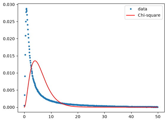
Clearly not the case at all. Which is to be expected, since there are many change pixels in
the scene and we have made no attempt to discriminate them.
In fact, it is easy to show that \\(Z\\) is a *likelihood ratio test statistic* for change, see
the discussion of statistical hypothesis testing in the
[SAR Tutorial](https://developers.google.com/earth-engine/tutorials/community/detecting-changes-in-sentinel-1-imagery-pt-2)
and the discussion on pp.390-391 in
[Canty (2019)](https://www.taylorfrancis.com/books/image-analysis-classification-change-detection-remote-sensing-morton-john-canty/10.1201/9780429464348).
Under the hypothesis that no change has occurred, the test statistic \\(Z\\) will follow, as we
said, a chi-square distribution. The so-called \\(p\\)-*value* is a measure of the extent to which
this is true. For an observation \\(z\\) of the test statistic, the \\(p\\)-value is the probability
that any sample drawn from the chi-square distribution could be as large as \\(z\\) or larger.
This is given by
$$ p(z) = 1-P_{\\chi\^2;N}(z),\\quad 0 \< p(z) \< 1, $$
where \\(P_{\\chi\^2;N}(z)\\) is the cumulative chi-square probability distribution, i.e., the area
under the chi-square distribution up to the value \\(z\\), and \\(p(z)\\) is its complement.
All \\(p\\)-values are equally likely if no change has occurred at that pixel
location\\(\^\\star\\), but **change will always be associated with small \\(p\\)-values** .
Therefore in order to eliminate the change observations from the MAD transformation,
the \\(p\\)-value itself can be used to weight each pixel before re-sampling the images to
determine the statistics for the next iteration. (This was the motivation for coding
a *weighted* covariance matrix routine in Part 1 earlier). The influence of the
change observations on the MAD transformation is thereby gradually reduced. Iteration
continues until some stopping criterion is met, such as lack of significant change in
the canonical correlations \\(\\rho_i\\). The whole procedure constitutes the *iMAD algorithm*.
It is implemented in the GEE Python API in the following cell:
\\(\\star\\) Thus the \\(p\\)-value is *not* a no-change probability, a common misapprehension!
See again the [SAR Tutorial](https://developers.google.com/earth-engine/tutorials/community/detecting-changes-in-sentinel-1-imagery-pt-2).
### The iMAD code
def chi2cdf(Z,df):
'''Chi-square cumulative distribution function with df degrees of freedom.'''
return ee.Image(Z.divide(2)).gammainc(ee.Number(df).divide(2))
def imad(current,prev):
'''Iterator function for iMAD.'''
done = ee.Number(ee.Dictionary(prev).get('done'))
return ee.Algorithms.If(done, prev, imad1(current, prev))
def imad1(current,prev):
'''Iteratively re-weighted MAD.'''
image = ee.Image(ee.Dictionary(prev).get('image'))
Z = ee.Image(ee.Dictionary(prev).get('Z'))
allrhos = ee.List(ee.Dictionary(prev).get('allrhos'))
nBands = image.bandNames().length().divide(2)
weights = chi2cdf(Z,nBands).subtract(1).multiply(-1)
scale = ee.Dictionary(prev).getNumber('scale')
niter = ee.Dictionary(prev).getNumber('niter')
# Weighted stacked image and weighted covariance matrix.
centeredImage, covarArray = covarw(image, weights, scale)
bNames = centeredImage.bandNames()
bNames1 = bNames.slice(0, nBands)
bNames2 = bNames.slice(nBands)
centeredImage1 = centeredImage.select(bNames1)
centeredImage2 = centeredImage.select(bNames2)
s11 = covarArray.slice(0, 0, nBands).slice(1, 0, nBands)
s22 = covarArray.slice(0, nBands).slice(1, nBands)
s12 = covarArray.slice(0, 0, nBands).slice(1, nBands)
s21 = covarArray.slice(0, nBands).slice(1, 0, nBands)
c1 = s12.matrixMultiply(s22.matrixInverse()).matrixMultiply(s21)
b1 = s11
c2 = s21.matrixMultiply(s11.matrixInverse()).matrixMultiply(s12)
b2 = s22
# Solution of generalized eigenproblems.
lambdas, A = geneiv(c1, b1)
_, B = geneiv(c2, b2)
rhos = lambdas.sqrt().project(ee.List([1]))
# Test for convergence.
lastrhos = ee.Array(allrhos.get(-1))
done = rhos.subtract(lastrhos) \
.abs() \
.reduce(ee.Reducer.max(), ee.List([0])) \
.lt(ee.Number(0.0001)) \
.toList() \
.get(0)
allrhos = allrhos.cat([rhos.toList()])
# MAD variances.
sigma2s = rhos.subtract(1).multiply(-2).toList()
sigma2s = ee.Image.constant(sigma2s)
# Ensure sum of positive correlations between X and U is positive.
tmp = s11.matrixDiagonal().sqrt()
ones = tmp.multiply(0).add(1)
tmp = ones.divide(tmp).matrixToDiag()
s = tmp.matrixMultiply(s11).matrixMultiply(A).reduce(ee.Reducer.sum(), [0]).transpose()
A = A.matrixMultiply(s.divide(s.abs()).matrixToDiag())
# Ensure positive correlation.
tmp = A.transpose().matrixMultiply(s12).matrixMultiply(B).matrixDiagonal()
tmp = tmp.divide(tmp.abs()).matrixToDiag()
B = B.matrixMultiply(tmp)
# Canonical and MAD variates.
centeredImage1Array = centeredImage1.toArray().toArray(1)
centeredImage2Array = centeredImage2.toArray().toArray(1)
U = ee.Image(A.transpose()).matrixMultiply(centeredImage1Array) \
.arrayProject([0]) \
.arrayFlatten([bNames1])
V = ee.Image(B.transpose()).matrixMultiply(centeredImage2Array) \
.arrayProject([0]) \
.arrayFlatten([bNames2])
iMAD = U.subtract(V)
# Chi-square image.
Z = iMAD.pow(2) \
.divide(sigma2s) \
.reduce(ee.Reducer.sum())
return ee.Dictionary({'done': done, 'scale': scale, 'niter': niter.add(1),
'image': image, 'allrhos': allrhos, 'Z': Z, 'iMAD': iMAD})
The following code cell is a routine to run the iMAD algorithm as an export task,
avoiding memory and time limitations in the active runtime. The asset will be exported
to the location specified by the `EXPORT_PATH` variable defined earlier. It requires
about 130 MB of space and can take 15 to 20 minutes to complete. Earth Engine
provides the asset for use in this demo, so it is not required that you run the
export cell to complete the tutorial.
### Run iMAD algorithm as export task
def run_imad(aoi, image1, image2, assetId, scale=20, maxiter=100):
try:
N = image1.bandNames().length().getInfo()
imadnames = ['iMAD'+str(i+1) for i in range(N)]
imadnames.append('Z')
# Maximum iterations.
inputlist = ee.List.sequence(1, maxiter)
first = ee.Dictionary({'done':0,
'scale': scale,
'niter': ee.Number(0),
'image': image1.addBands(image2),
'allrhos': [ee.List.sequence(1, N)],
'Z': ee.Image.constant(0),
'iMAD': ee.Image.constant(0)})
# Iteration.
result = ee.Dictionary(inputlist.iterate(imad, first))
# Retrieve results.
iMAD = ee.Image(result.get('iMAD')).clip(aoi)
rhos = ee.String.encodeJSON(ee.List(result.get('allrhos')).get(-1))
Z = ee.Image(result.get('Z'))
niter = result.getNumber('niter')
# Export iMAD and Z as a single image, including rhos and number of iterations in properties.
iMAD_export = ee.Image.cat(iMAD, Z).rename(imadnames).set('rhos', rhos, 'niter', niter)
assexport = ee.batch.Export.image.toAsset(iMAD_export,
description='assetExportTask',
assetId=assetId, scale=scale, maxPixels=1e10)
assexport.start()
print('Exporting iMAD to %s\n task id: %s'%(assetId, str(assexport.id)))
except Exception as e:
print('Error: %s'%e)
and here we run it on our two images:
asset_path = f'{EXPORT_PATH}LandkreisOlpe'
run_imad(aoi, im1.select(visirbands), im2.select(visirbands), asset_path)
```
Exporting iMAD to projects/YOUR_GEE_PROJECT_NAME/assets/imad/LandkreisOlpe
task id: None
```
After the export finishes (if you ran it), the number of iterations and the
final canonical correlations can be read from properties of the exported image.
(Earth Engine-hosted assets are imported here, edit the paths if you'd like to
use your copies)
im_imad = ee.Image(
'projects/google/imad_tutorial/LandkreisOlpe').select(0, 1, 2, 3, 4, 5)
im_z = ee.Image(
'projects/google/imad_tutorial/LandkreisOlpe').select(6).rename('Z')
niter = im_imad.get('niter').getInfo()
rhos = ee.List(im_imad.get('rhos')).getInfo()
print('iteratons: %i'%niter)
print('canonical correlations: %s'%rhos)
```
iteratons: 28
canonical correlations: [0.9981250148930833,0.9818308995435004,0.9594475307384785,0.8816514687633029,0.8470795072417497,0.6869925605138704]
```
We got convergence after 28 iterations, and the correlations are very close to one
for the first canonical variates. It might now be interesting to check if the test
statistic \\(Z\\) has the expected chi-square distribution when evaluated for the no
change pixels. To to eliminate the changes at the 10% significance level we set a
lower threshold of \\(\\alpha = 0.1\\) on the \\(p\\)-values (recall: small p-values signify change).
scale = 20
# p-values image.
pval = chi2cdf(im_z, 6).subtract(1).multiply(-1).rename('pval')
# No-change mask (use p-values greater than 0.1).
noChangeMask = pval.gt(0.1)
hist = im_z.updateMask(noChangeMask).reduceRegion(ee.Reducer \
.fixedHistogram(0, 50, 500), aoi, scale=scale, maxPixels=1e11) \
.get('Z').getInfo()
a = np.array(hist)
x = a[:, 0] # array of bucket edge positions
y = a[:, 1]/np.sum(a[:, 1]) # normalized array of bucket contents
plt.plot(x, y, '.', label = 'data')
plt.plot(x, chi2.pdf(x, 6)/10, '-r', label='chi2(6)')
plt.legend()
plt.show()
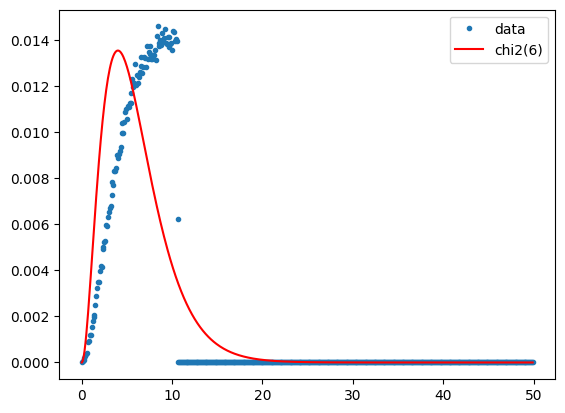
Agreement is not perfect, but the plot is certainly closer to the ideal chi-square distribution
after iteration than after the single MAD transformation. So let's display the *iMAD* image:
M1 = geemap.Map()
M1.centerObject(aoi, 11)
display_ls(im1.select(visbands), M1, 'im1')
display_ls(im2.select(visbands), M1, 'im2')
display_ls(im_imad.select('iMAD1', 'iMAD2', 'iMAD3'), M1, 'iMAD123', True)
M1
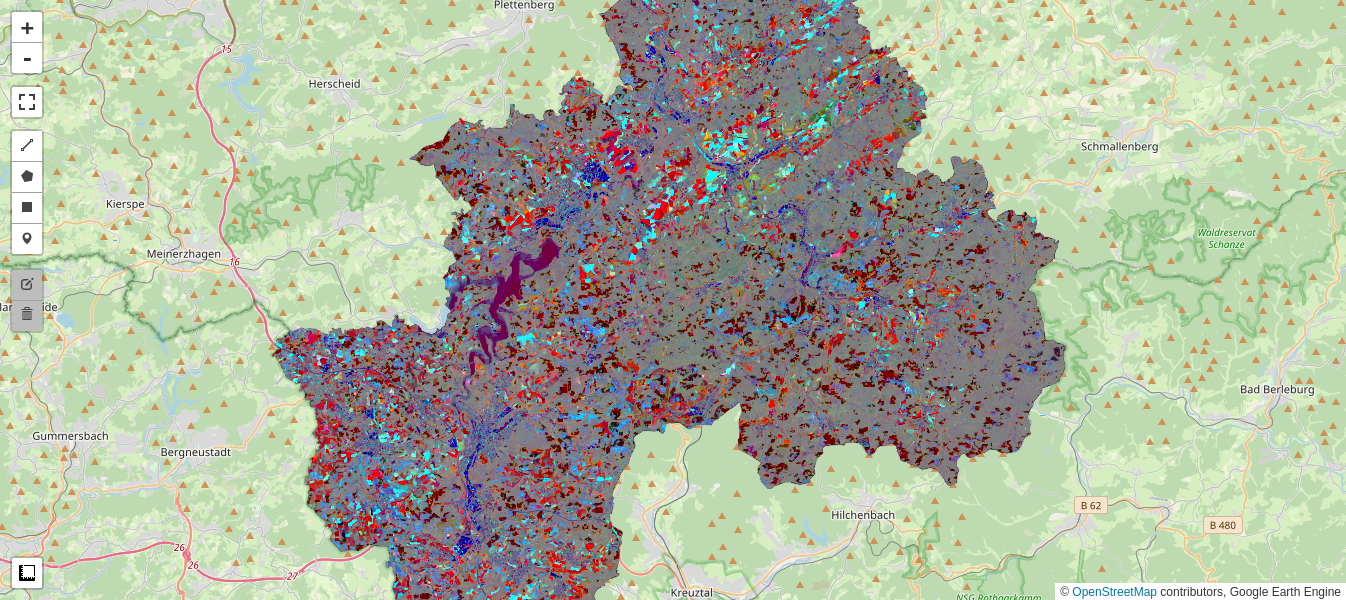
Gray pixels point to no change, while the wide range of color in the iMAD variates
indicates a good discrimination of the types of change occurring.
**Aside:** We are of course primarily interested in extracting the changes in the iMAD
image, especially those which mark clear cutting, and we'll come back to them in a moment.
However, now that what we think the no change pixels have been isolated, we could
also perform a regression analysis on them to determine how well the radiometric parameters
of the two Sentinel-2 acquisitions compare. If surface rather than top of atmosphere (TOA)
reflectance images had been used for the example, we would expect a good match, i.e., a
slope close to one and an intercept close to zero at all spectral wavelengths. In general,
for uncalibrated images, this will not be the case. In that event, the regression
coefficients can be applied to normalize one image (the target, say) to the other
(the reference). This might be desirable for tracing features such as NDVI indices over
a time series of acquisitions when the images have not been reduced to surface reflectances,
see e.g., [Gan et al. (2021)](https://ieeexplore.ieee.org/document/9392311), or indeed for
*harmonizing* the data from two different sensors of the same family such as Landsat 7 with
Landsat 8. These topics will be the subject of Part 3.
But now let's look in more detail at the changes in the Landkreis Olpe scene.
### Clustering
To better interpret the change image, we can attempt an unsupervised classification.
We'll see if we can get away with an ordinary K-means clusterer and a simple Euclidean distance
measure for the complete iMAD image. We choose the number of clusters as 4 and leave all 12(!)
other input parameters of the *wekaKmeans()* clusterer at their default values. We will also
first standardize the iMAD image by dividing by the square root of the variances of the no-change
pixels, \\(\\sigma_i = \\sqrt{2(1-\\rho_i)},\\ i=1\\dots 6\\). This will favour a more compact
no-change cluster.
# Standardize to no change sigmas.
sigma2s = ee.Image.constant([2*(1-x) for x in eval(rhos)])
im_imadstd = im_imad.divide(sigma2s.sqrt())
# Collect training data.
training = im_imadstd.sample(region=aoi, scale=scale, numPixels=50000)
# Train the clusterer.
clusterer = ee.Clusterer.wekaKMeans(4).train(training)
# Classify the standardized imad image.
result = im_imadstd.cluster(clusterer)
Here we display the four clusters overlaid onto the two Sentinel 2 images:
M2 = geemap.Map()
M2.centerObject(aoi, 13)
display_ls(im1.select(visbands), M2, 'im1')
display_ls(im2.select(visbands), M2, 'im2')
cluster0 = result.updateMask(result.eq(0))
cluster1 = result.updateMask(result.eq(1))
cluster2 = result.updateMask(result.eq(2))
cluster3 = result.updateMask(result.eq(3))
palette = ['red', 'yellow', 'blue', 'black']
vis_params = {'min': 0, 'max': 3, 'palette': palette}
M2.addLayer(cluster0, vis_params, 'new clearcuts')
M2.addLayer(cluster1, vis_params, 'agriculture')
M2.addLayer(cluster2, vis_params, 'prior clearcuts')
M2.addLayer(cluster3, vis_params, 'no change')
M2
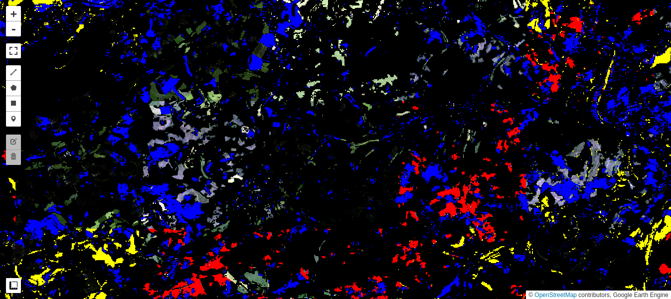
### Interpretation
**Cluster 0** (colored red in the preceding map) appears to classify the clear
cuts occurring over the observation period quite well.
**Cluster 1** (yellow) marks changes in the agricultural fields and pastures.
**Cluster 2** (blue) is more ambiguous but can be mainly associated with changes
in previously cleared forest (seasonal or new growth) as well as with some changes
in agricultural fields and in built up areas.
**Cluster 3** (black) is no change.
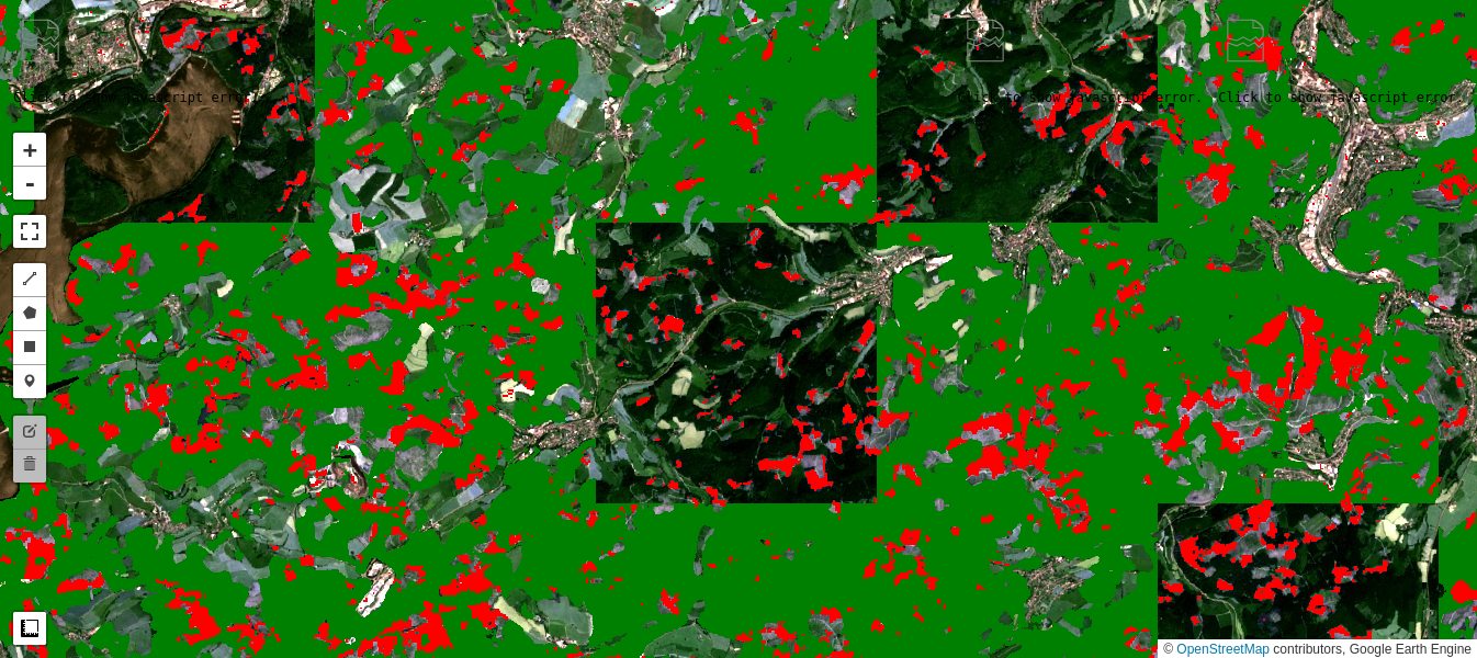
### Comparison with Dynamic World
Google's recently released [Dynamic World](https://developers.google.com/earth-engine/tutorials/community/introduction-to-dynamic-world-pt-1)
dataset contains near real-time land use land cover predictions created from Sentinel-2
imagery for nine land use land cover classes including forest (trees class). It is interesting
to compare the loss in forest cover as determined from our iMAD/Cluster pipeline with the
Dynamic World tree map for the comparable time period. In the code snippet below, we gather
an image collection covering our observation period and simply mosaic them. The *mosaic()*
method composites the overlapping images according to their order in the collection (last on top),
which is what we want because the changes in tree cover are occurring over the entire period.
Generally the agreement is excellent, although the iMAD change map registers a number of
small-area clear cuts missed in the Dynamic World map:
dyn = ee.ImageCollection('GOOGLE/DYNAMICWORLD/V1') \
.filterDate('2021-06-01', '2022-06-30') \
.filterBounds(aoi) \
.select('label').mosaic()
# 'trees' class = class 1
dw = dyn.clip(aoi).updateMask(dyn.eq(1))
M3 = geemap.Map()
M3.centerObject(aoi, 13)
display_ls(im1.select(visbands), M3, 'im1')
display_ls(im2.select(visbands), M3, 'im2')
M3.addLayer(dw, {'min': 0, 'max': 1, 'palette': ['black', 'green']}, 'dynamic world')
M3.addLayer(cluster0, vis_params, 'new clearcuts')
M3
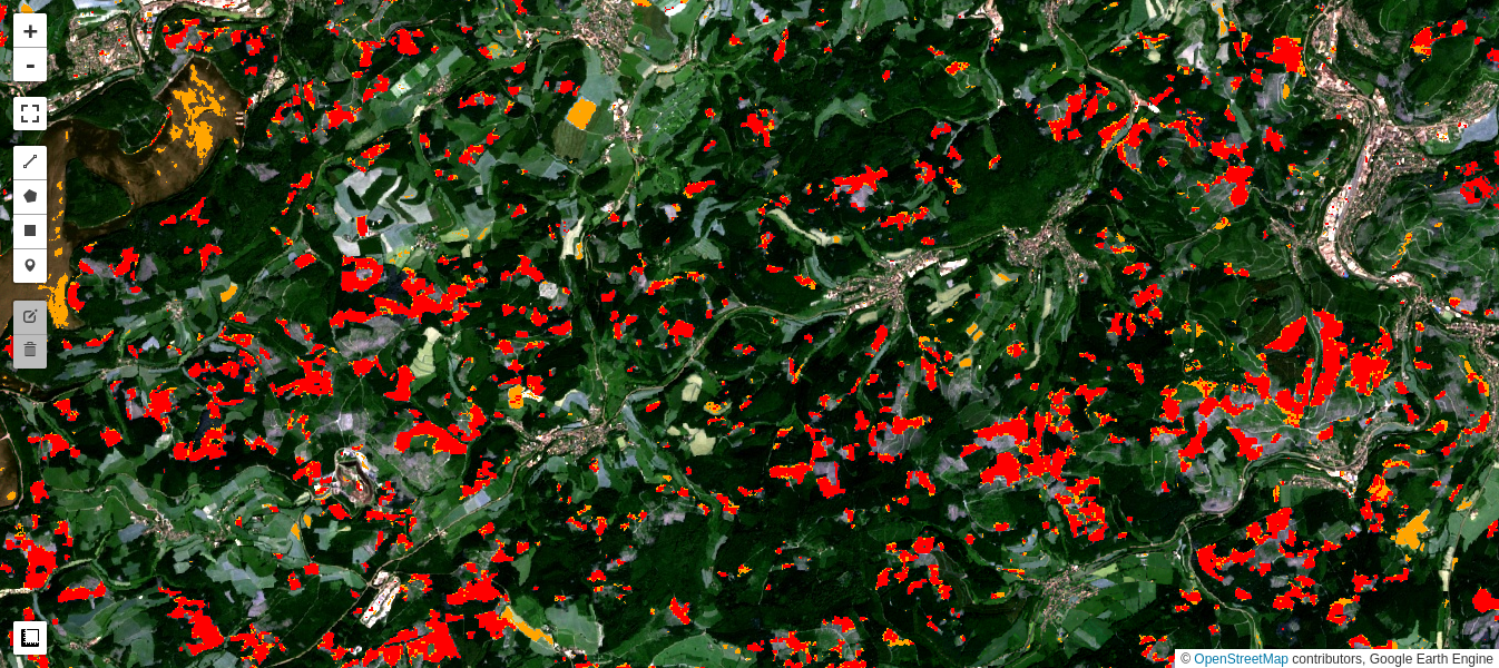
### Simple difference revisited
In fact, K-means clustering of the simple difference image also gives a fairly good discrimination
of the clear cuts. This is because the NIR band is especially sensitive to all vegetation changes,
and is also only weakly correlated with the other five bands. However, close inspection indicates
that there are many more false positives, especially in agricultural fields, as well as in the reservoir.
M4 = geemap.Map()
M4.centerObject(aoi, 13)
diff = im1.subtract(im2).select(visirbands)
training = diff.sample(region=aoi, scale=20, numPixels=50000)
clusterer = ee.Clusterer.wekaKMeans(4).train(training)
result1 = diff.cluster(clusterer)
cluster0d = result1.updateMask(result1.eq(0))
display_ls(im1.select(visbands), M4, 'im1')
display_ls(im2.select(visbands), M4, 'im2')
M4.addLayer(cluster0d, {'min': 0, 'max': 3,
'palette': ['orange', 'yellow', 'blue', 'black']}, 'clearcuts (diff)')
M4.addLayer(cluster0, vis_params, 'clearcuts (iMAD)')
M4
### Deforestation quantified
From the clear cuts class number 0, and using the *pixelArea()* function, we can extract the
total area cleared between June 2021 and June 2022 within the Landkreis Olpe, whereby we
exclude small areas covering less than 0.2 hectare:
# Minimum contiguous area requirement (0.2 hectare).
contArea = cluster0.connectedPixelCount().selfMask()
# 0.2 hectare = 5 pixels @ 400 sq. meters.
mp = contArea.gte(ee.Number(5)).selfMask()
# Clear cuts in hectares.
pixelArea = mp.multiply(ee.Image.pixelArea()).divide(10000)
clearcutArea = pixelArea.reduceRegion(
reducer=ee.Reducer.sum(),
geometry=aoi,
scale=scale,
maxPixels=1e11)
ccA = clearcutArea.get('cluster').getInfo()
print(ccA, 'hectare')
```
4401.391057999339 hectare
```
The most recent [commercial forest inventory](https://www.it.nrw/itnrw) recorded for
the Landkreis Olpe as of December 2019 was 40,178 hectare, so we have determined that,
allowing for further decreases in 2020 and the first half of 2021, more than 9.3% of
woodland was lost to drought/clearing within the time period measured.
Finally, repeating the calculation with the clear cuts determined with the simple difference image:
contArea = cluster0d.connectedPixelCount().selfMask()
mp = contArea.gte(ee.Number(5)).selfMask()
pixelArea = mp.multiply(ee.Image.pixelArea()).divide(10000)
clearcutArea = pixelArea.reduceRegion(
reducer=ee.Reducer.sum(),
geometry=aoi,
scale=scale,
maxPixels=1e11)
ccA = clearcutArea.get('cluster').getInfo()
print(ccA, 'hectare')
```
3992.8200707562282 hectare
```
thus overestimating the loss from clear cutting by about one third.
## Summary
In Part 2 of this tutorial, we have generalized the MAD transformation to an iterative scheme,
the iMAD algorithm. Then, we illustrated change detection with the algorithm by focussing a
particular application, namely detection of clear cutting of coniferous trees destroyed by
drought in an administrative district in Germany.
While simple image comparison or differencing can be useful, the statistical transformations
implicit in the iMAD algorithm offer a more powerful means of analyzing and categorizing changes
in bitemporal image data. In Part 3, we will examine the use of iMAD for image calibration tasks,
giving some examples of relative radiometric normalization over an image sequence, as well as
harmonization of reflectances from different sensors.
## Exercises
1. Try another parameter set, or one of the other clusterers in the GEE arsenal to see if you can
improve on the above classification.
2. In the discussion up till now we have not included the Sentinel-2 red edge bands. Repeat the
analysis with all 10 visual/infrared bands:
visirbands + rededgebands
```
['B2', 'B3', 'B4', 'B8', 'B11', 'B12', 'B5', 'B6', 'B7', 'B8A']
```
1. Determine with the aid of a cloud-free S2 image from summer, 2020 the forest cover loss in the
district for the 2-year period ending June 2022.
2. Urban and suburban sprawl accompany the growth of many large cities. If they are located in at
least partly forested areas, deforestation due to new housing and infrastructure development can
be very rapid and widespread. An extreme example is the city of Houston, Texas, where massive
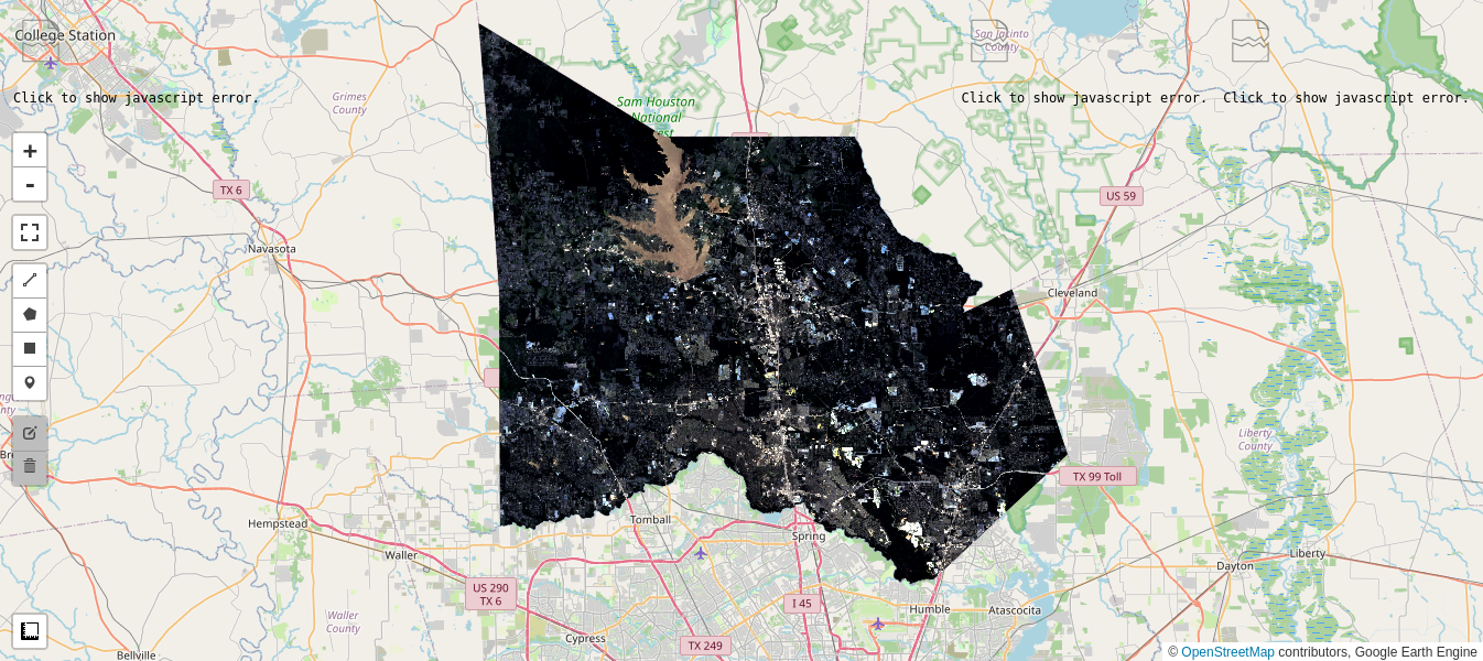
encroachment on the surrounding coutryside is a recognized problem. Below is an area of interest
comprising Montgomery County, which encompasses heavily wooded areas to the north of the city,
and two cloud-free Sentinel-2 images from July 2021 and June 2022. Repeat the analysis with
the iMAD/Cluster pipeline to determine the loss of woodland within the County over that time
period. (Hint: Since a variety of mad-made changes occur in the scene, the interpretation of
unsupervised classification of the change image is critical.)
# TIGER---: US Census Counties from the GEE Data Archive.
counties = ee.FeatureCollection('TIGER/2016/Counties')
filtered = counties.filter(ee.Filter.eq('NAMELSAD', 'Montgomery County'))
aois = filtered.geometry()
# There are many Montgomery Counties in USA, we want the 12th in the list.
aoi = ee.Geometry(aois.geometries().get(12))
im1, im2 = collect(aoi, '2021-07-01', '2021-07-30', '2022-06-01', '2022-06-30')
M5 = geemap.Map()
M5.centerObject(aoi, 10)
display_ls(im1.select(visbands), M5, 'Image 1')
display_ls(im2.select(visbands), M5, 'Image 2')
M5
```
Sun Jul 25 17:15:25 2021
```
```
Sat Jun 25 17:15:27 2022
```